Tutorial 7
Problem Statement
Automatic process control is well established in many applications ranging from large refineries using multivariate model-based control to climate control of buildings using simple on/off control. Wastewater treatment plants are no exception. The implementation of even basic automatic control should improve performance and save money. In GPS-X, the user can simulate the effects of automatic process control.
To improve and stabilize operation, as well as realize energy savings, you decide to implement MLSS and dissolved oxygen control. You will do this by incorporating MLSS and DO controllers into your system.
Objectives
This tutorial will show you how to set up a dissolved oxygen controller that automatically changes the aeration rate to meet the dissolved oxygen set point.
This tutorial also will show you how to set up an MLSS controller to automatically adjust the biosolids wastage rate to meet the specified MLSS set point.
Using an Automatic DO Controller
1. Open the layout completed in Tutorial 2 and save it as `tutorial-7’.
2. Switch into Simulation Mode if not already there.
3. Open the Flow Controls’ properties tab by right clicking on an empty space on the input control tab and pressing the Input Control Properties… button. Set the influent flow slider maximum to 7,500 m3/d. Press Accept.
4. Check that the DO Controller is activated. By default, the aeration tank is set up to use a DO controller, but we will just confirm that it is selected. Within the Simulation mode for the Aeration Tank go to Input Parameters > Operational. In the Aeration Setup section, the specify oxygen transfer by… variable should be set to Using a DO Controller. If it is not, switch to modelling mode, change the value and come back to simulation mode.
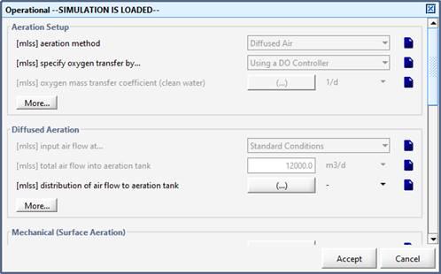
Figure 7‑1 – Check that DO Controller is On
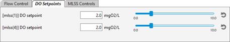
5. Create new input controls. On a new input tab, you will create sliders for two of the DO setpoints. The setpoints can be accessed from the aeration tank’s Input Parameters > Operational form under the Aeration Control section.
Click the ellipsis button (…) beside the DO setpoint label to access the individual array elements.
Drag the first and last DO setpoint array elements to the input control tab to create the sliders.
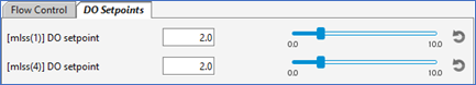
Figure 7‑2 – DO Setpoint Input Controllers
6. Create a new output graph. Make a new output graph tab and call it ‘Controller Response’. You will be adding the dissolved oxygen concentration in the first and fourth reactors of the plug-flow tank and the effluent ammonia nitrogen.
Right-click on the aeration tank and select the Output Variables > Concentrations in Reactors. Beside the dissolved oxygen in reactors label click the ellipsis button (…) to access the individual array elements. Drag the first and last elements to a new graph (both elements are to be contained in the same graph).
Right-click on the aeration tank’s effluent stream (not the tank itself). Select Output Variables > Concentrations and drag ammonia nitrogen (under the Nitrogen Compounds section) to the graph.
7. Edit the graph settings. Change the max value for all the y-axes to 10 (the same as the DO setpoint slider limit) and give the graph a proper title.
8. Auto Arrange the graphs.
9. Save the layout.
10. Run some 20-day simulation, varying the influent flowrate and the DO setpoints.
Using an Automatic MLSS Controller
Now we are going to add an MLSS controller to the layout to automatically adjust the biosolids wastage rate to meet the specified MLSS set point.
Setting up an Automatic MLSS Controller
11. Switch to Modelling Mode.
12. Locate the control variable. This will be the MLSS in the aeration tanks’s effluent stream. We will need to discover the cryptic name (ie. the internal “short form” variable name within GPS-X calculations) of this variable so that we can identify this variable later.
Right-click on the aeration tank’s effluent stream (not the tank itself) and select Output Variables > Concentrations. You should see a form like Figure 7‑3.
Hover the mouse pointer over the label for mixed liquor suspended solids and a tooltip should appear. The tooltip has the form label/cryptic. From this, we can see that the cryptic name of the variable is xmlss. Remember this value for later.
Alternatively, you can right-click on the label for mixed liquor suspended solids and select “Copy Cryptic Name to Clipboard”. This will store xmlss on your computer’s clipboard so that you can paste it into a field later.
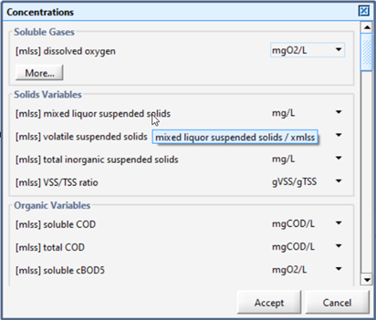
Figure 7‑3 – Viewing Cryptic Variable Name
13. Identify the manipulated variable. The most logical variable for this is the wastage flowrate, which in this case, is the pumped flow from the clarifier.
14. Turn on the controller. Access the clarifier's Input Parameters > Operational data entry form. You will be changing a couple of values in this dialog.
Under the Pumped Flow section, turn on the controller and set the setpoint for control variable to 2000.
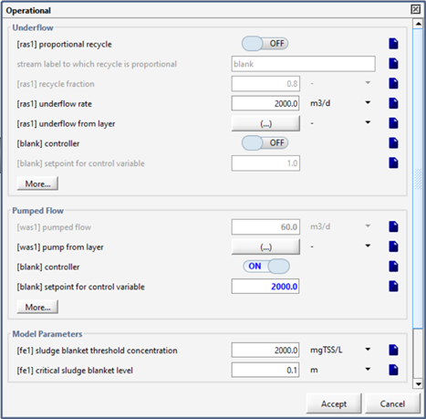
Figure 7‑4 – Clarifier’s Operational Dialog (Pumped Flow)
15. Define the control variable. At the bottom of the Pumped Flow section (see figure above), click the More… button to access the controller’s settings (Figure 7‑5). Make the following changes:
a. replace blank with xmlss in the control variable field (use Ctrl-V to paste the cryptic name if you had previously saved it to the clipboard)
b. enter 0.05 days as the controller sampling time (this represents the frequency with which the controller samples the control variable, or MLSS in this case)
c. turn OFF the controller effect on control variable - direct. This means that the manipulated variable, the wastage flow rate, is increased to reduce the control variable, MLSS. (A different control loop such as air flow and DO concentration would require the controller effect on control variable - direct switch to be turned ON as an increase in the manipulated variable, air, would result in an increase in the control variable, DO). (ie. Turn OFF for an inverse relationship and turn ON for a proportional relationship)
d. enter 200 m3/d as the maximum pumped flow
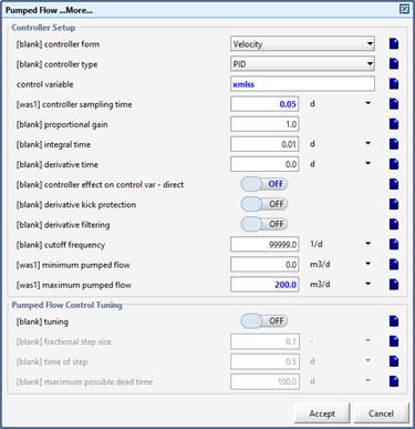
Figure 7‑5 – MLSS Controller Settings
16. Accept the forms.
17. Save the Layout.
Tuning the Automatic MLSS Controller
18. Switch to Simulation Mode.
19. Create a new input tab. You will be adding 5 input controllers to the tab.
These settings can be found by going to the clarifier’s Input Parameters > Operational > Pumped Flow main form and within the Pumped Flow More… form.
· controller on/off
· setpoint for control variable (set limits from 0 to 4000)
· proportional gain (set limits from 0 to 50)
· integral time (set limits from 0 to 10)
· derivative time (set limits from 0 to 10)
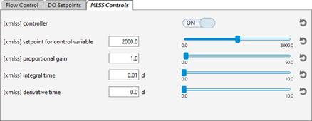
Figure 7‑6 – MLSS Input Controls
20. Create a new graph. Add the following three variables to the same graph:
· the mixed liquor suspended solids (from the aeration tank’s effluent stream Output Variables > Concentrations form)
· the influent flow (from the influent’s Output Variables > Flow form)
· the wastage flow (from the clarifier’s pump stream Output Variables > Flow form)
21. Edit the graph properties. Change the max values of the y-axis to 7500 (influent flow), 5000 (mlss), and 600 (wastage flow).
Note that you may have to ‘unlock’ the max fields so that you can edit the values individually (click the lock icon beside the Max label).
Give the graph an appropriate title.
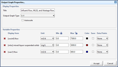
Figure 7‑7 – Graph Properties
22. Create a scenario. Call it “Sinusoidal” and change the influent flow type to sinusoidal and keeping the influent flow as the default 2000.0 m3/d (Tutorial 3 - Using Scenarios for instructions if needed).
23. Save the layout.
24. Run a 10-day dynamic simulation with sinusoidal scenario and the controller turned ON.
Initially, you will find that the manipulated variable, the wastage flow rate, oscillates wildly between its minimum and maximum values. This is a controller tuning problem. It is usually possible to obtain reasonable controller performance by trial and error. In this example, one may conclude that the controller gain is too large. One option for tuning this controller by trial-and-error is as follows:
· Start with a low proportional gain (0.001), high integral time (10 days), and low derivative time (0 days). This creates a sluggish but stable controller.
· Watch how the wastage rate changes to counteract the effect of a disturbance (e.g. influent flow rate). If it does not react quickly enough, try increasing the proportional gain. Continue to increase the proportional gain until you get a reasonably responsive control effect, but still a stable response.
· If the wastage rate becomes unstable (wild oscillations) decrease the proportion gain.
· With the proportional effect stable, try decreasing the integral time to increase the performance of your controller.
· If there is too much overshoot, try increasing the derivative time
A simplified understanding of the three elements of a PID controller is: fast, persistent and predictive for the P, I and D terms, respectively. Remember that automatic process control is not a simple subject, and it may not be possible to achieve the level of control that you desire. Consider the process time constant of the MLSS in the aeration basin. It takes several days for a plant to reach a new steady-state given a change in wastage rate, while the plant upsets (changes in the influent flow rate) that can have a dramatic effect on the MLSS can occur in a matter of hours or even minutes.
There are several published approaches for finding good initial tuning constants for PID controllers. One approach is to use the Ciancone correlations (Marlin, 1995[4]) which are included in GPS-X's PID tuning tool. The Ciancone correlations provide the tuning constants given the gain, time constant, and dead time of the process, under the assumption that the process dynamics may be represented with reasonable accuracy by a first-order plus dead time model. In GPS-X's PID tuning tool, the process response to a step change in the manipulated variable is fit to a first-order plus dead time model using least squares (in tuning mode). The Ciancone correlations are then used to determine the appropriate values for the tuning constants.
25. Create another scenario. Base it on the Sinusoidal scenario (so that it has the influent flow type from that scenario) and call it “Tuning”.
26. Activate the pumped flow control tuning mode.
Browse to the clarifier’s Input Parameters > Operational form. Click the Pumped Flow section’s More button and find the Pumped Flow Control Tuning section.
Turn the tuningswitch ON. Also drag this variable to the input control tab so that it can be easily turned OFF in the future.
The fractional step size can be specified on that form and can be a positive or negative value. In this case, set the fractional step size to 0.5.
Accept the More dialog to return to the Operational form.
Now (under the Pumped Flow section) turn the controller OFF and set the pumped flow value to 100 m3/d.
This fractional step size corresponds to a step in pumped flow rate from 100 m3 /d to 150 m 3/d.
Acceptthe Operational form.
27. Double-check that you have the right settings. Select Scenario > Show from the Simulation Toolbar to see all the variables that you have changed for this scenario. You should see a dialog similar to Figure 7‑8.

Figure 7‑8 – Scenario Show Dialog
28. From the input controls tab, turn the MLSS controller ON and run a 0-day steady state simulation with the newly created scenario.
29. Now, turn the MLSS controller OFF using the ON-OFF control switch[5] and run a 10-day dynamic simulation.
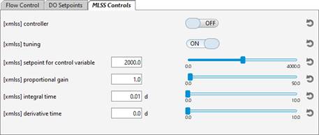
![]()
Figure 7‑9 - Input Controller Setting
The simulation performed in tuning mode is shown in Figure 7‑10. The essential characteristics of a successful tuning mode simulation are:
· It must be started under steady state, with values of the manipulated (pumped flow) and controlled (MLSS) variables representative of normal operating conditions.
· The simulation should last long enough to capture most of the process dynamics (i.e. the simulation should end at steady-state, or be approaching steady-state), and
· The step in the manipulated variable should be large enough to dominate other "noise" that affects the controlled variable (in this case the sinusoidal influent flow pattern).
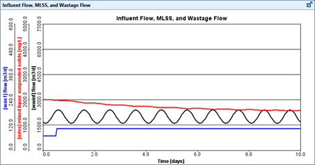
Figure 7‑10 – Tuning Mode Simulation
At the end of the simulation, PID tuning constants will be calculated (this may take several seconds), and will appear in the Command Window (see Figure 7‑11).
|
|
The Command Window can be opened by selecting this option from the Simulation Control button, located at the bottom of the screen, on the Simulation Toolbar. Scroll to the bottom of the Command Window for the xmlss settings displayed in Figure 7‑11. |
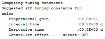
Figure 7‑11 – Calculated PID Tuning Constants
30. Create another scenario. Base it on the Tuning scenario (so that it starts with all the variables from that scenario) and call it “MLSS Control”.
31. Change the input controller values. In the input control tab, set the proportional gain, integral time, and derivative time to the values shown in the Command Window. Also turn ON the MLSS controller and turn OFF the tuning mode.
|
|
32. Transfer the controller values to the scenario. Press the “Transfer controls to scenario” button on the Controls toolbar and add the controller tuning constants to the scenario to store these settings. |
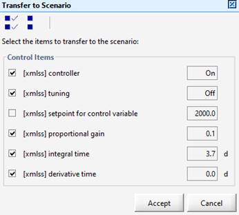
Figure 7‑12 – Transfer to Scenario
33. Save the layout.
34. Run a 10-day dynamic simulation. The results shown in Figure 7‑13 were performed using these tuning parameters for the MLSS controller. The MLSS setpoint was 2000 mg/l and the average influent flow rate was decreased to test the performance of the controller under dynamic conditions.
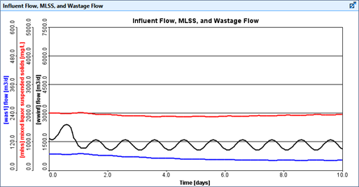
Figure 7‑13 – Simulation with MLSS Controller