Tutorial 6
Problem Statement
You are interested in testing your plant under more dynamic or stressful conditions such as a storm. Unfortunately, you do not have access to real storm flow data. Therefore, you will generate a simulated storm loading to your plant and then input this data as a driving function for the model. You will investigate the effect of step feed during the storm.
Interactive controllers provide an easy-to-use method for exploring the dynamic response of the model. However, in most modeling projects, it is desirable if not essential to input real forcing functions to examine how the model behaves under real conditions. The forcing functions can be flows or influent concentrations, or any other model parameter, but are always in the form of time dynamic data; that is, variable values over time. A typical set of time dynamic data would be the influent flow rate to the plant over a period of time. GPS-X facilitates the input of this data so that the model will be tested against real conditions.
Objectives
This chapter covers an important and useful feature of GPS-X:
· Using a data file as an input to control simulations
Setting up Dynamic Input
1. Open the layout built in Tutorial 2 and save it as `tutorial-6’ using File > Save As...
2. Switch to Simulation Mode.
3. Create Input Controllers. More information regarding input controllers is presented in Tutorial 2. Right-click on the influent and select Composition > Influent Characterization to bring up the Influent Advisor tool.
The Influent Advisor will take up most, if not all, of the room on the main window. Click the little right arrow (see Figure 6‑1) between the “User Inputs” column and “State Variables” column to shrink the window and hide everything except the “User Inputs” column.
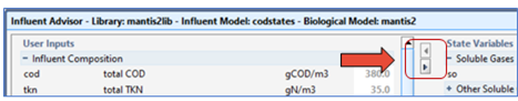
Figure 6‑1 – Shrink Influent Advisor
Now that you have room, drag total COD, total TKN and ammonia nitrogen to the controls section to create interactive sliders.
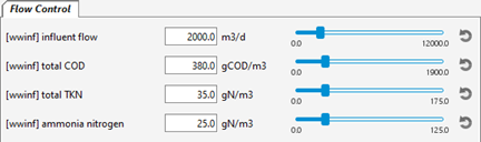
Figure 6‑2 – New Input Controllers
The next step is setting up the data in files to be read by GPS-X during a simulation. There are two different ways that data files can be prepared for the file input controllers:
A. Manually preparing spreadsheets outside of GPS-X (best used for preparing data for multiple variables) and adding the data file to the layout in Scenario > Configuration.
or
B. Using the Data File… tool in the GPS-X to automatically prepare the file (best used for preparing data for a single variable).
This tutorial will use both methods to illustrate their use.
Method A: Manually Preparing a Spreadsheet Input File
4.
![]() To open the Data File organizer window,
press the Data File button on the main toolbar in GPS-X.
To open the Data File organizer window,
press the Data File button on the main toolbar in GPS-X.
5. Press the New button to open the Data File Creation Wizard.
6. Ensure Input Variable is selected in the ‘Input or Output’ pane of the Data File Creation Wizard. Press Next.
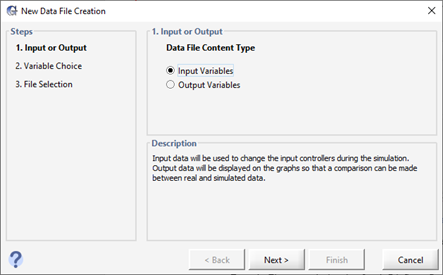
Figure 6‑3 – Data File Creation Wizard
7. Select the Variables. All the input variables that are currently used to make an input controller will be available to add to a data file.
From the Flow control tab, select [wwinf] influent flow, [wwinf] total COD, [wwinf] total TKN and [wwinf] ammonia nitrogen. Press Next.
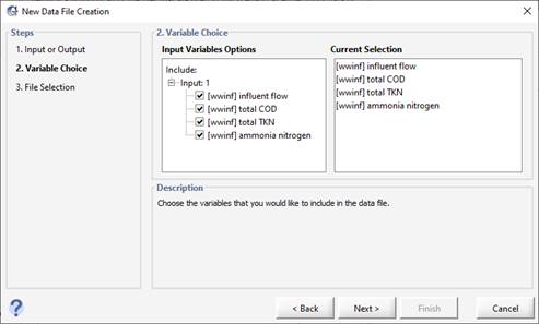
Figure 6‑4 - Input Variable Selection
8. Save the File. By default, GPS-X will save the excel sheet in the active directory with the same name as the layout. Press Finish.
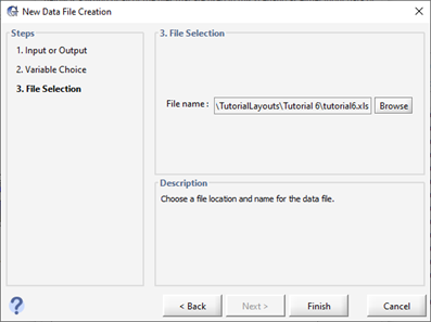
Figure 6‑5 - Save New Data File
9. Open the file. You will be prompted to open the new file after saving it. Press Yes.
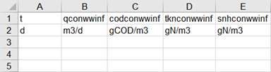
Figure 6‑6 - Input Data File Generated by GPS-X
We have created a version of this data file that has already been populated with data to use for this portion of the tutorial. Locate and open the tutorial-6-example-data.xls spreadsheet file in the following subdirectory of the GPS-X installation:
\layouts\08tutorials\
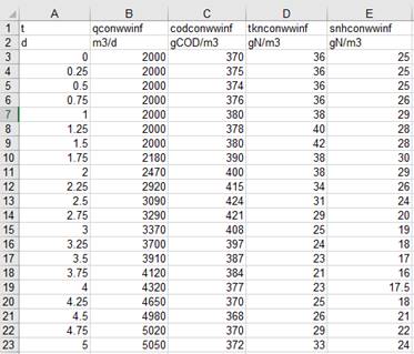
Figure 6‑7 – Contents of “tutorial-4-example-data.xls”
We will use the data found in this file as our dynamic dataset. It is a typical set of influent input data that you might use to simulate a change in influent loading over time.
The first column is labeled “t” for time, and is in the units of days “d.”
The remaining columns contain data for each of the parameters being read from the file. The names at the head of each column are the “cryptic variable name” (which is the internal “short form” variable name within GPS-X calculations) for each variable. These names are specific to the layout you have created and are different for each variable and object within the layout. The units of the data reported in the column are then specified in the row after the cryptic name. The units can be different than the units used by the input controller, as long as the units are recognized by GPS-X. All the units recognized for a given input variable can be viewed by opening the unit drop down menu next to the variable in the input control properties window.
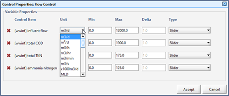
Figure 6‑8 - Available Influent Flow Units
Note that if any data was missing from the data file presented in Figure 6‑7, a question mark (?) can be entered in the cell corresponding to the missing data point and GPS-X will continue to use the last value assigned to that variable.
10. Verify that the cryptic names in the data file are the same as the variables for the input controllers. The simplest way to do this is to look at the tooltip that pops up when you hover the mouse cursor over the controller’s label as shown in Figure 6‑9.
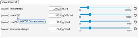
Figure 6‑9 – Viewing the Cryptic Name via Tooltip
The cryptic variable names for the four variables used in this tutorial are:
qconwwinf – influent flow
codconwwinf – total COD
tknconwwinf – total TKN
snhconwwinf – ammonia nitrogen
If the variables you are interested in are not currently on an input controller, you can quickly find the cryptic variable name by using the GPS-X find functionality. You can access the find function by going to Edit > Find on the main tool bar or using CTRL-F.
This will open the Find pop-up window. In the ‘Find Input/Output Variable’ pane of the find window there is an input box with a toggle for Keyword and Cryptic beneath it.
If you need to find a cryptic variable name and you know part of its plain English variable name, type it in the entry field and select, for example ‘total COD’. Ensure the keyword option is selected and press find. This will find and display every variable in the model that contains the keywords ‘total COD’. The matching variables will be grouped by the object they are associated with. The stream associated with the variable will be given in front of the variable name.
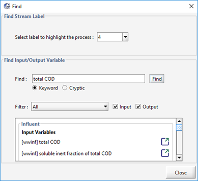
Figure 6‑10 - Finding all Instances of total COD in the Model
If a variable is related to a stream number/name that you do not recognize, use the ‘Select label to highlight the process’ drop down menu in the ‘Find Stream Label’ pane to select the stream. This will highlight the object that the stream initiates from on the layout. For example, selecting the stream ‘mlss’ from the drop-down menu will highlight the Aeration tank.
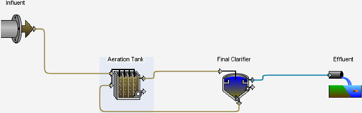
Figure 6‑11 - Using the Find Stream Label Functionality to Identify where the mlss Stream Originates
|
|
After identifying the variable of interest under the influent > Input Variables headings you can click on the Go to location button to the right of the variable to be taken to the window where this variable is defined. Hovering the cursor over the variable name will cause a tooltip containing the cryptic variable name to appear. |
Alternatively, if you are given a cryptic variable name by a GPS-X output, the corresponding plain English variable name can be identified using the find functionality. For example, after opening the find window, select the cryptic option and enter the cryptic variable name codconwwinf in the find field. Pressing the Find button will present you with input and output variable which have a cryptic name containing codconwwinf.
|
Note that “wwinf” in the cryptic variable name above comes from the label for the influent stream (eg. if you had labeled the influent stream as “1”, the cryptic name for influent flow will show up as “qcon1”). |
11. Access the Configuration window. Click on the Scenario menu on the Simulation Toolbar and select Scenario > Configuration/Data Files… > Data Files.
![]()
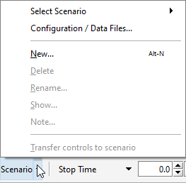
Figure 6‑12 - Accessing Scenario > Configuration/ Data Files…
Access the list of current data files. The configuration window will show all the scenarios available (in this case it should just be the Base Model). Data files can be added to a specific scenario if desired by selecting it before pressing the Data Files button. Make sure Base Model is selected and press the Data Files button.
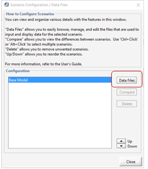
Figure 6‑13 – Scenario Configuration showing Data Files button
12. Add the data file. The Data Files window shows all the files that this scenario is currently using. At this point, there will not be any files displayed. To add the Excel file prepared above, press the Add button and browse to the appropriate location and select the tutorial-6-example-data.xls file.

Figure 6‑14 – Adding File to Scenario
13. Accept the changes and close the Scenario Configuration window. Notice that the interactive slider for the inputs have automatically changed to file input controls that cannot be directly edited. The values are now being read in from the file.
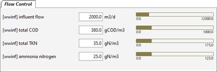
Figure 6‑15 – Controllers Changed to File Input
14. Run a 5-day simulation with Steady-State click ON. As the simulation proceeds, the values of the influent flow and concentration will change in the input controller. The model responds dynamically to the changing input, as shown in the increasing effluent solids.
Method B: Using the GPS-X Data File Tool
The above methodology is useful for simulations where data for many parameters are being read in simultaneously, and it is easy to assemble that data externally in a spreadsheet.
There is another option that is useful for simple simulations where just one or two parameters are being read from a file, and you want to input those values directly into GPS-X. For this situation, you can use the Data File Tool.
15. Create another Input Controller. Right-click on an open spot in the layout background and select System > Input Parameters > Physical Environment Settings. Drag liquid temperature to a new input tab (i.e. drop it in a blank area beside the current tab’s label). This will create a new slider controller on a new tab.
16. Rename the tab to “Temperature”.
17. Access the Data File tool for this input. Right-click on controller’s label (liquid temperature) and select the Data File… option. A new window will be displayed.
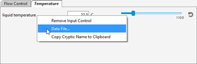
Figure 6‑16 – Accessing Data File Tool
18. Enter the data from Table 6‑1. Select a cell in the table and type the value. Using the tab key, you can move to the next cell.
Table 6‑1 - Data for Liquid Temperature Controller
|
t [d] |
temp [C] |
|
1 |
17 |
|
2 |
18 |
|
3 |
20 |
|
4 |
22 |
|
5 |
24 |
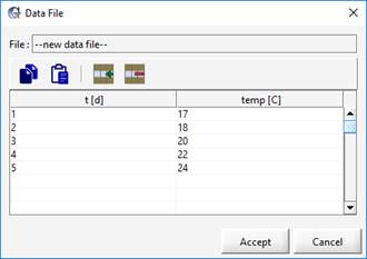
Figure 6‑17 – Data File Tool with Values
19. Save the data by pressing Accept. You will be prompted to save the file. The default location is the same directory as the layout file and the default name is the layout’s name with the cryptic name of the variable concatenated to it. These defaults are usually appropriate, so click Save to save the file.
Notice that the interactive slider for the liquid temperature input has automatically changed into a file input control bar and is no longer able to be manually adjusted.
20. Run a 5-day simulation with Steady-State clicked ON. As the model is simulated, the value of influent flow, concentrations and temperature will change in the input controller.
Plotting Measured Data along with Simulated Results
The previous section described the method for importing input data to the simulation file. In this section, the method for importing and displaying the measured output data onto a graph alongside simulated results will be introduced. This is convenient for comparing the measured value from a plant with the simulated results given in GPS-X. It also makes it easier to calibrate and optimize the process (see Tutorial 10 for details regarding optimization).
21. Create a spreadsheet file with example measured data. The table below is an example of the observed total suspended solids data for the final effluent from our example plant. Create a data file with this information and save it in the same directory as the layout file.
Table 6‑2 – Measured Data
|
t |
xfe1 |
|
d |
mg/L |
|
0 |
12 |
|
1 |
11.8 |
|
2 |
13.7 |
|
3 |
18 |
|
4 |
25 |
|
5 |
28 |
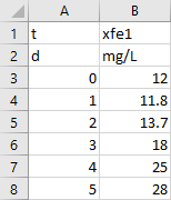
Figure 6‑18 - Excel Spreadsheet with Values
The cryptic variable name for the total suspended solids in the final effluent (xfe1) can be found by right-clicking on the output graph created in Tutorial 2 and selecting Output Graph Properties… from the drop-down menu. Hold the mouse cursor over the variable label and a tooltip will appear with the label/cryptic information as shown in Figure 6‑19. This should correspond to the name on the first row of the spreadsheet file.
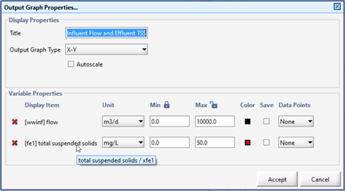
Figure 6‑19 – Tooltip showing Cryptic Variable Name
22. Add the data file. Following the same procedure as the last section where we added an input data file to the layout, access Scenario > Configuration/Data Files… > Data Files and add this new file to the layout.
23. Run a 5-day simulation with Steady-State clicked ON. The data points from the measured data are shown as diamond-shaped points on the graph, as shown in Figure 6‑20.
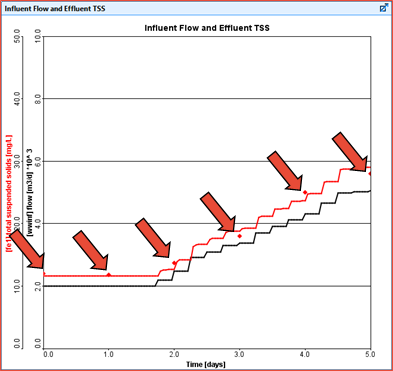
Figure 6‑20 – Graph showing Measured Data Points
Statistical Analysis of the Models Performance
A statistical analysis can then be conducted within GPS-X to test the model’s ability to reproduce the observed data. Statistical Analysis can only be preformed on X-Y timeseries output plots that have data points displayed on the plot.
24. Run a 5 Day Simulation.
25. Open the Statistics Menu. Right click anywhere on the graph and select the statistics > [fe1] total suspended solids option.
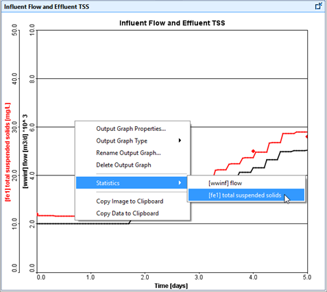
Figure 6‑21 – Accessing the Statistics Menu for Total Suspended Solids
26. Select the Statistical Analysis. The statistics option will provide you with a variety of Model Fit and Residual Analysis that can be conducted.
From the Model Fit Evaluation section of the menu, select:
· Plot of simulated vs measured
· Table of goodness-of-fit residuals
From the ‘Residuals Analysis’ section, under the ‘plot against measured values’ heading, select:
· Residuals
Note: The measured data section of the statistical analysis allows you to specify the method in which the data has been collected. The Grab Data option assumes that the data represented on the plot was collected at that specific point in time. For more details on the measured data types available, refer to the Technical Reference manual.
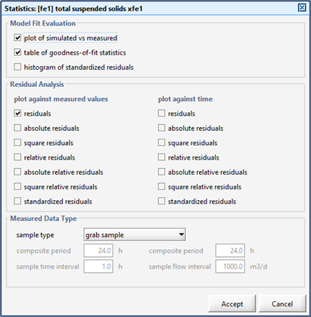
Figure 6‑22 – Selecting the Statistical Analysis to be Preformed on the Model
Note: For full details on the calculation of all the statistical analysis available in GPS-X, refer to the Technical Reference manual.
27. Press Accept. GPS-X will automatically produce the selected plots on the current output tab. Press the Auto Arrange button on the Output too lbar to view all the plots.
Using the data presented in the output plots, you can judge the ability of your model to represent data collected from your plant. If you are not satisfied with the statistical analysis, further manipulation to influent advisor and your object settings may be required. You can use input controllers to fine tune your model within Simulation Mode.
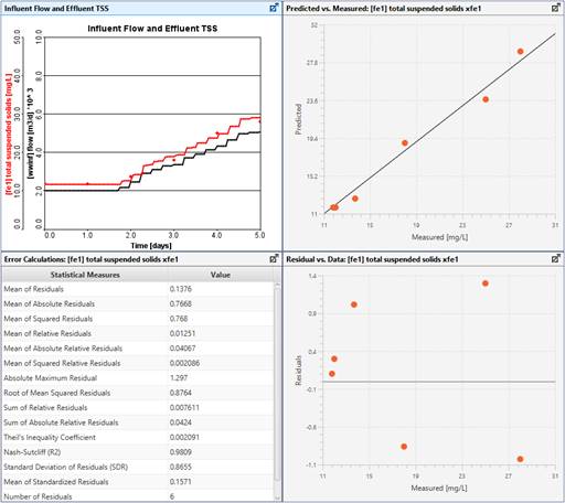
Figure 6‑23 – Results of the Total Suspended Solids Statistical Analysis
Creating a Bar Chart for Steady-State Condition
The measured data of distributions within a unit can also be plotted along with the simulated result as a bar chart. The methodology for doing so is similar to the previous section.
28. Create a new blank output tab by clicking on the New Graph Tab button on the output toolbar.
29. Create a new graph. For this example, we will use the variable for readily degradable soluble substrate in reactors within the plug-flow tank. Right-click on the plug-flow tank and select Output Variables > Concentrations in Reactors form and within the sub-heading Organic Variables select theMore… form. Drag the “readily degradable soluble substrate in reactors” variable under the Other Soluble Organic Compounds sub-heading to the new tab area. Since it is an array of values, the default graph type is a bar chart.
|
|
30. To open the Data File organizer window, press the Data File button on the main toolbar in GPS-X. |
31. Press the New button to open the Data File Creation Wizard.
32. Select Output Variables in the ‘Input or Output’ pane of the Data File Creation Wizard. Press Next.
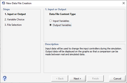
Figure 6‑24 - Select Output Variables in the Data File Creation Wizard
33. Select the Variables. All the output variables that are currently on an output graph will be available to add to a data file.
Select the following variables:
· [mlss(1)] readily degradable soluble substrate in reactors
· [mlss(2)] readily degradable soluble substrate in reactors
· [mlss(3)] readily degradable soluble substrate in reactors
· [mlss(4)] readily degradable soluble substrate in reactors
Or simply select:
· [mlss] readily degradable soluble substrate in reactors
Note the brackets containing numbers beside the cryptic variable name. This represents the reactor number within the aeration tank. The default number of reactors is four.
34. Press Next.
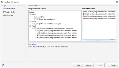
Figure 6‑25 - Select the Output Variables to be Included in the Data File
35. Press Finish to save the File. When prompted to open the new Excel sheet press Yes.
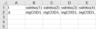
Figure 6‑26 - Output Variable Data File Created by Data File Creation Wizard
36. Use the data in the table below to populate the Data File. Save the Excel Sheet.
Table 6‑3 – Measured Data for Aeration Tank
|
t |
sslmlss(1) |
sslmlss(2) |
sslmlss(3) |
sslmlss(4) |
|
d |
mgCOD/L |
M gCOD/L |
mgCOD/L |
mgCOD/L |
|
0 |
2.8 |
1.68 |
1.21 |
0.88 |
37. Add the data file. Following the same procedure as the previous section where we added an input data file to the layout, access Scenario > Configuration / Data Files and add this new file to the layout.
38. Autoscale the Bar Chart. Press the ‘Output Properties’ button on the Outputs toolbar and select the Autoscale feature for the Bar Chart.
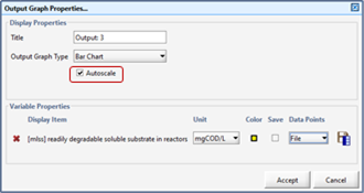
Figure 6‑27 – Autoscale the Bar Chart
39. Rename the output graph. Right on graph and select Rename Output Graph…. Enter an appropriate title for the output graph, such as “Readily Degradable Soluble Substrate Distribution”, and click OK.
40. Run a 0-day simulation with Steady-State clicked ON. The data from the Excel file should show up with the simulated result as a bar chart, as shown in Figure 6‑28.
Notice that the simulated result is shown as a colored bar chart and the measured data is shown as a meshed bar chart.
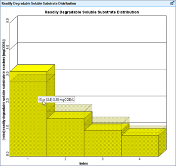
Figure 6‑28 – Bar Chart showing Measured Data
Clicking on a bar will display the measured data (in square brackets) followed by the simulated data value.
41. Save the layout.