Tutorial 8
Problem Statement
Some important operational variables in a wastewater treatment plant are site specific and difficult to generalize. These variables include sludge residence time (SRT) and food-to-microorganism ratio (F/M). In addition, other calculations, such as daily averages, moving averages, and mass flows are applied to most water quality parameters throughout the plant. Consequently, it is desirable for any wastewater treatment plant model to contain these traditional process variables, and GPS-X provides you with this capability.
Objectives
This tutorial will show you how to define operational variables such as SRT.
In addition, mathematical operations such as averaging, and flux calculations will be demonstrated.
These operations are centered around the Define function (Tools > Define menu or the Define button located on the main toolbar).
Setting up the Layout
1. Create a new layout consisting of:
· A wastewater influent object,
· a control splitter,
· a plug-flow tank,
· a rectangular secondary clarifier
· a 2-flow combiner
· a wastewater outfall
Use the mantis2lib library and the default model selections (codstates influent model, the mantis2 plug flow tank model and the simple1drectangular clarifier model).
Connect the unit processes and add the labels as displayed in Figure 8‑1. The control-splitter unit process will be used to simulate a bypass weir.
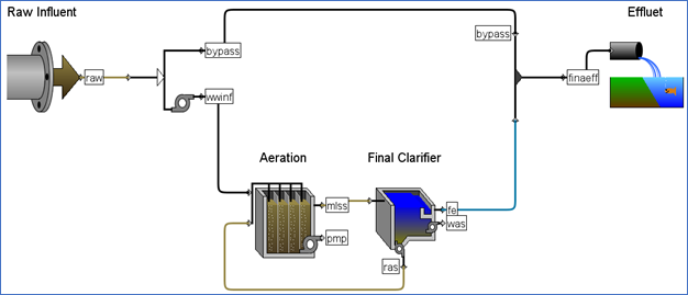
Figure 8‑1 – Tutorial 8 Layout
2. Modify the clarifier underflow parameters. Access the Input Parameters > Operational data entry form and change the following settings:
· Turn ON the proportional recycle.
· Beside stream label to which recycle is proportional change “blank” to “wwinf” (ie. the influent stream to the aeration tank).
· The recycle fraction is already 0.8 which is acceptable for this example.
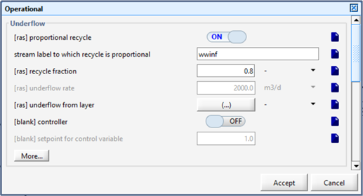
Figure 8‑2 – Modify Underflow Settings
3. Modify the clarifier pumped flow. In the same data entry form (scroll down if necessary) change the pumped flow (which will be used as the wastage rate) from 40 m3/d to 100 m3/d.
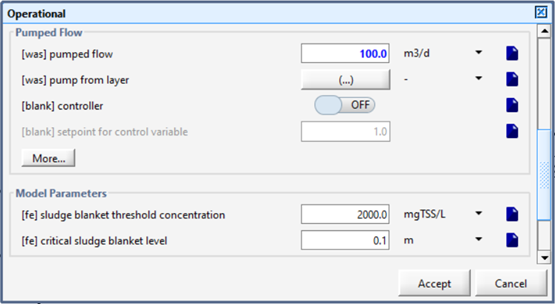
Figure 8‑3 – Modify Pumped Flow
4. Accept these changes and save the layout.
Defining Mass Flows
Now that the layout has been set up, we will define a mass flow variable of the effluent solids. This mass flow is defined as the effluent suspended solids multiplied by the effluent flow rate.
5. Access the Define Wizard. Click on Define button on the main toolbar and select Mass Flow from the options.
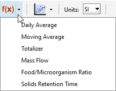
Figure 8‑4 – Mass Flow in the Define Wizard Submenu
6. Select the streams (as shown in Figure 8‑5):
· Control Splitter > bypass
· Final Clarifier > fe
· 2-flow Combiner > finaleff
7. Select the variable. As shown in Figure 8‑5, select Composite Variables > total suspended solids.
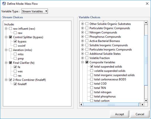
Figure 8‑5 – Define Mass Flow Wizard
8. Press Accept and then save the layout.
Now that the variable has been defined, we will set up a graph and run a simulation to view the results.
9. Switch to Simulation Mode.
10. Create a new graph. You will be adding three mass flow variables to this graph.
Right-click on the clarifier fe connection point and select the Output Variables > Defined Variables > Mass Flow.
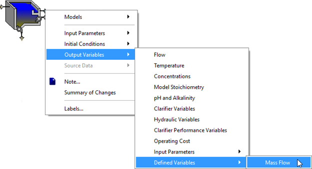
Figure 8‑6 - Accessing the Defined Variables
Drag the Mass Flow.total suspended solids variable to an output graph.
Repeat this procedure for the bypass and the finaleff streams so that all three mass flows are displayed on the same output graph.
11. Modify the graph settings. Set the max axis values on that graph to 1,000 kg/d and set the title to “Mass Flows”.
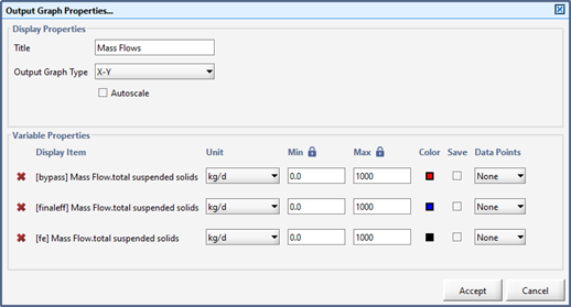
Figure 8‑7 - Mass Flow Graph Settings
12. Create an input controller for the influent flow rate. As described in Tutorial 2 set up the controller and set the maximum flow to 6,000 m3/d.
13. Auto Arrange the graph and run a 20-day dynamic simulation.
14. Increase the influent flow rate and notice that when the influent flow rate is above 2000 m3/d (the default pump flow rate for the Control Splitter object), some flow will begin to bypass the plant and show up in the bypass stream. An example is displayed in Figure 8‑8. Note that your output graph will look different when compared to the figure below depending on the adjustments you make to the slider during the simulation run.
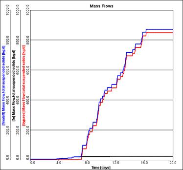
Figure 8‑8 – Mass Flow Output Graph
15. Try changing the bypass flow limit by increasing the pumped flow rate in the Control Splitter object. To prevent having to recompile the model, this must be done either by defining a scenario or by placing the bypass pump flow on an input controller. For instance, to create an input controller, right-click on the control splitter and go to Input Parameters > Pumped Flow and add pumped flow as an input controller. Set the maximum pumped flow to 6,000 m3/d.
16. Re-run the simulation and try to reduce the total mass flow of solids discharged to the receiving water.
17. Save the layout.
Defining an SRT
In this section, you will learn how to calculate and display SRT, the solids residence time in the system.
18. Switch to Modelling Mode.
|
|
19. Access the SRT Manager window. Click on Define button on the main toolbar and select Solids Retention Time from the options. |
|
|
20. Create a new SRT Variable. Click the green ‘+’ button and enter ‘tank’ as the name for the variable (Note: the full name will be ‘srttank’ because ‘srt’ is automatically prepended to all variable names). |
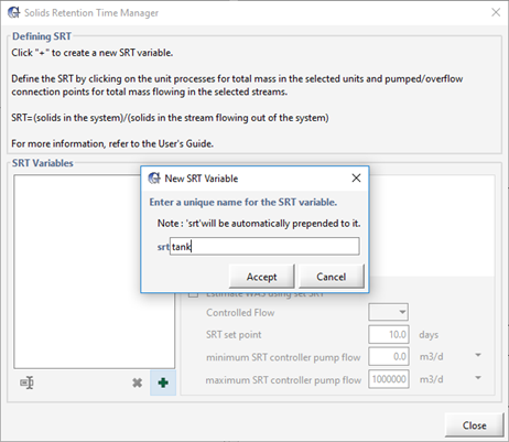
Figure 8‑9 – Create a New SRT Variable
21. Accept the name. A new blank SRT equation will be shown on the right side of the window.
22. Define the equation. This process involves clicking on the appropriate locations on the drawing board while keeping the SRT Manager window open. You may have to move the SRT Manager window in order to access everywhere that you need.
There are two parts to the SRT equation: Mass()/Mass Flow()
I. The numerator is the mass section of the equation, and it includes the mass of solids held in each tank. Typically, SRT calculations only include the mass of solids held in the aeration basin, but it is also possible to calculate SRT by summing the mass in the aeration basin and the final clarifier. While the SRT equation is shown, every time you click on a tank the mass of solids in that unit process will be included in the SRT calculation.
Click the following processes to add them to the numerator:
|
|
· Aeration Tank (since this process represents several reactors, you will be prompted for which ones you’d like to include. Include all of them.) · Clarifier |
II. The denominator part of the equation is the excess solids mass flow lines that are used to calculate SRT. This is done by pointing to the flow lines which convey solids out of the system. Typically, this will only include the waste flow.
Click the following connection points to add them to the denominator:
|
|
· was · fe |
The equation should now look like the following:
Mass(mlss,fe)/Mass Flow(was,fe)
However, for this example, we will not be including the clarifier’s mass in the calculation.
23. Remove the clarifier’s mass. Click on the clarifier again to remove it from the equation.
Mass(mlss)/Mass Flow(was,fe)
24. Close the SRT Manager window to accept the equation.
25. Save the layout.
26. Switch to Simulation Mode.
27. Create a graph with the SRT variable. In Simulation Mode, when you open the SRT Manager from the Define menu, you can only view the SRT variables and their equations. You can also drag the variable’s label from this window to a new or existing graph. Drag the ‘srttank’ variable to a new graph tab.
Note: This will add two variables to the graph. The instantaneous and dynamic SRT. Depending on the need, one or the other can be removed. In our case, we will just leave both.
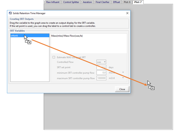
Figure 8‑10 – Dragging SRT Variable to a Graph
28. Modify the graph properties. Change the y-axis max value to 30 days and change the graph title to “SRT”.
29. Save the layout.
30. Try running a few simulations, observing the SRT as you change the amount of solids being wasted out of the system. Do this by adding an input controller for the [was] pumped flow from the secondary clarifier through right-clicking on the ‘was’ output and going to Input Parameters > Operational.
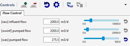
Figure 8‑11 – Update Set of Input Controllers
Defining Averages
The procedure for defining averages is similar to setting up mass flow calculations. In addition, averaging calculations can also be applied to a defined mass flow, SRT, or F/M ratio. Here, you will apply averaging calculations to the Mass Flow in the discharge stream defined above.
31. Switch to Modelling Mode.
|
|
32. Access the Define Wizard. Click on Define button on the main toolbar and select Daily Average from the options. |
33. Change the Variable type to “Define Variables.”
Select the desired variable(s). In this case, we will only select 2-flow Combiner > finaleff > Mass Flow > Mass Flow.total suspended solidsas shown in Figure 8‑12.
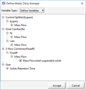
Figure 8‑12 – Define Daily Average Wizard
34. Press Accept and then save the layout.
You have now set up a daily average calculation for the mass flow of suspended solids in the “finaleff” stream.
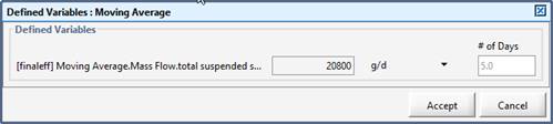
35. Define a moving average for the Mass Flow.total suspended solids in the “finaleff” stream.Use the same procedure as above except select Moving Average instead of Daily Average from the Define menu.
36. Press Accept and then save the layout.
37. Switch to Simulation Mode.
38. Create a new graph. You will be adding the new daily and moving averages variables to this graph.
Right-click on the combiner’s finaleff connection point and select the Output Variables > Defined Variables > Daily Average and drag the variable to a blank area to create the graph. Do the same with the Moving Average variable and add it to the same graph.
|
NOTE: You will notice in the display form for the Moving Average variable that a number will appear to the right of the variable name. This number represents the number of days that are used in each moving average calculation. You must be in Modelling mode to edit this # of Days value.
Figure 8‑13 – Moving Average # of Days |
39. Change the graph properties. Set a maximum limit of 1,000 kg/d for both variables and set the title to “Daily and Moving Average Flows”.
40. Run the model and change the influent flow rate to observe the moving and daily averages. For example, running the model with the following controller settings provides the graph displayed in Figure 8‑14. Note that your output graph will look different depending on how the control slider for the influent flow is adjusted during the simulation.
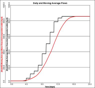
Figure 8‑14 – Moving and Daily Averages Output Graph
Controlling SRT with Waste Pump Rate
When defining a SRT equation, you have the option to create a process controller for SRT. This controller will adjust the waste flow rate to achieve a given SRT set point.
41. Switch to Modelling Mode.
42. Set the SRT controller. Bring up the SRT Manager window. Select an SRT to control (for this example select srttank) and click on the Estimate WAS using set SRT option, as shown below.
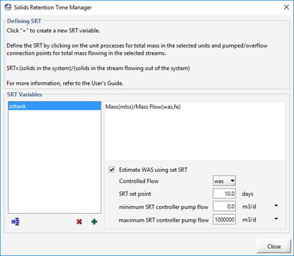
Figure 8‑15 – Estimating WAS using set SRT
43. Edit the settings. In this situation, we are just going to leave the values at their defaults, but in the settings section, you can choose the appropriate wastage flow to control and enter the desired SRT (in days) into the SRT set point field, as well as specify the min/max of the flow.
Only one SRT can be controlled at a time via this method. If multiple SRT controllers are required (e.g. for plants in parallel) then a PID control loop can be used in the pump control section of the secondary clarifier or a toolbox object. More information regarding PID controllers is presented in Tutorial 7.
44. Switch to Simulation Mode.
45. Create another input controller. Open the SRT Manager again (in Simulation Mode) and drag the SRT set point to the input controller tab to create a slider for that variable. Edit the settings and change the max value to 30 days.
At the same time, within the SRT Manager window drag the Estimate WAS using set SRT selection to the input controller tab to create an ON/OFF switch. If desired, this allows you to easily adjust this setting without having to open the SRT Manager in the Modelling mode. For the next steps, keep the use set point SRT to estimate waste flow to ON.
46. Create an output graph. To observe the required WAS flow rate while changing the SRT set point, we will create another graph (on the same tab as the SRT graph created in Step 27) that contains the WAS flow rate. It is accessed by clicking on the clarifier’s WAS connection point and selecting Output Variables > Flow. Edit the graph settings, change the max value of the y-axis to 500 m3/d and set the title to “Was Flow”.
47. Try running simulations at various SRT point values to observe required WAS flowrate to achieve the desired SRT. An example is shown below in Figure 8‑16. Note that your output will look different depending on how the SRT set point controller is adjusted during the simulation.
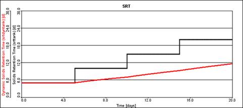
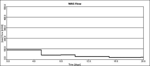
Figure 8‑16 – SRT and WAS Flow Output Graph