Tutorial 18
Problem Statement
Once a model has been calibrated, mathematical optimization can be employed to find the best operating conditions to achieve certain objectives such as minimizing net energy usage, total chemical usage or the overall operating costs. These objectives are directly impacted by numerous variables in the model which the user can set independently of the other variables in the model.
The Nelder-Mead Simplex method available in GPS-X is ideal when solving optimization problems with a small number of target and manipulated variables, but as the size of the problem increases, the algorithm can take a considerable amount of time to solve. A Data Driven Optimization (DDO) Method has been included in the GPS-X install that is ideal for optimization with many parameters. The computational time of this method is largely independent of the number of manipulated parameters in the optimization problem but rather depends on the complexity of the model and a defined number of maximum iterations.
In this tutorial, we will find the optimal operating conditions to minimize a plants net energy consumption under different operating conditions. We will be manipulating variables that have direct impact on the plant’s energy consumption while ensuring that the plant effluent quality is maintained within emission limits.
Objective
The purpose of this tutorial is to see how Python can be used to optimize the operating conditions used in GPS-X. By the end of this tutorial, you can use Python to solve complex optimization problems in a GPS-X layout.
Manipulated Variables
The following process variables will be available to be manipulated by the DDO algorithm in the specified range of settings:
Table 18-1 – Manipulated Variables in the DDO definition
|
Manipulated Variable Effluent Constraint |
Lower Bound |
Upper Bound |
Units |
|
Primary WAS |
0.0 |
100.0 |
m3/d |
|
Secondary WAS |
5.0 |
200.0 |
m3/d |
|
Aerobic 1 Recycle |
1000.0 |
10000.0 |
m3/d |
|
Aerobic 1 DO Setpoint |
1.0 |
4.0 |
mgO2/L |
|
Aerobic 2 DO Setpoint |
1.0 |
4.0 |
mgO2/L |
|
Ferric Dosage |
0.0 |
10.0 |
gFe/m3 |
|
RAS |
1000.0
|
2000.0 |
m3/d |
Operational Constraints
The following emission limits and operational constraints have been imposed on our treatment plant and must be observed:
Table 18‑1 - Plant Effluent Limits
|
Effluent Constraint |
Lower Bound |
Upper Bound |
Units |
|
Total Suspended Solids |
0.0 |
20.0 |
mg/L |
|
Total Carbonaceous BOD5 |
0.0 |
10.0 |
mgO2/L |
|
Total Nitrogen |
0.0 |
7.5 |
mgN/L |
|
Ammonia Nitrogen |
0.0 |
0.2 |
mgN/L |
|
Ortho-Phosphate |
0.0 |
0.1 |
mgP/L |
Table 18‑2 - Plant Operational Constraints
|
Operational Constraint |
Lower Bound |
Upper Bound |
Units |
|
Mixed Liquor Suspended Solids |
1500.0 |
5000.0 |
mg/L |
Creating an Objective Function
We will now look at how custom GPS-X code can be used to create an objective function. Alternatively, this could be obtained directly in Python by collecting each variable in the objective function and directly calculating the objective function.
1. Load the starting point layout. We’ve already set up a layout to be used for this tutorial. The layout can be found at File > Sample Layouts > Tutorials> Tutorial 18 (Starting Point).
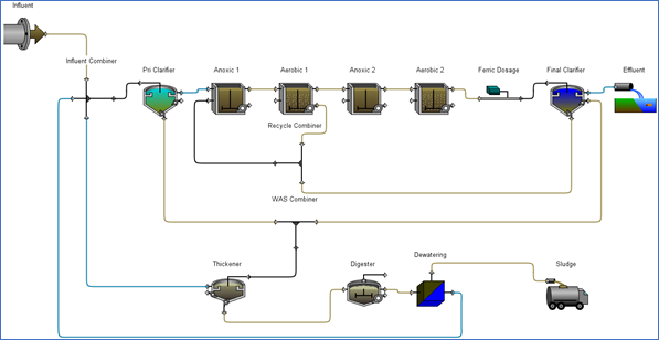
Figure 18‑1 - Tutorial 18 Layout
2. Save the Layout with a new name. We will be making changes to the layout and do not want to change the starting point layout.
3. Open the Macros User File. This can be opened by going to Layout > General Data > User Files > Macros…
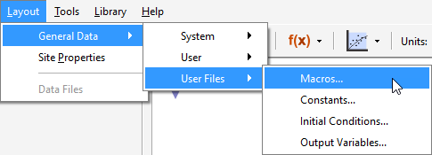
Figure 18‑2 - Accessing the Macro File
You will be adding code to the Derivative section of the Macro file.
4. Add Macro Code. You will be creating a single GPS-X variable to represent our objective function. Add the following code to the DERIVATIVE SECTION of the macro file to allow GPS-X to automatically calculate this variable.
netenergylayout = totalpowerkw - electricitySavedwdig/24.0
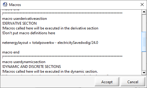
Figure 18‑3 - Updated Macro Code
The netenergylayout variable will be our optimization objective function. The calculation examines the difference between the instantaneous energy consumption (kW) in the plant and the estimated electricity that can be generated by the digester unit (kWh).
5. Click Accept in the Macros window to save the changes.
6. Create an Output Variable for the objective function. The custom Output Variables entry form can be found by going to Layout > General Data > User Files > Output Variables…
7. Add the following code to the output variable entry form:
display netenergylayout !Net Energy Used in the Layout !kW
8. Click Accept in the Output Variables window to save the changes.
9. Save the Layout and reload. This will cause GPS-X to read in the output variable and create a menu for it under Layout > General Data > User > Output Variables > User Defined Output Variables as displayed in Figure 18‑4.
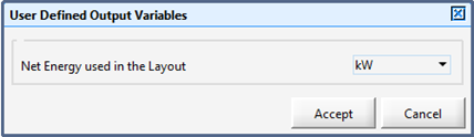
Figure 18‑4 - User Defined Output Variables Menu
10. Open Simulation Mode.
11. Create a Digital Type Output Graph containing the following variables:
· Layout > General Data > User > Output Variables > User Defined Output Variables > Net Energy used in the Layout
· Aerobic 2 effluent > Concentrations > Mixed Liquor Suspended Solids
· Effluent > Concentrations > Total Suspended Solids
· Effluent > Concentrations > total cBOD5
· Effluent > Concentrations > Ammonia Nitrogen
· Effluent > Concentrations > Total Nitrogen
· Effluent > Concentrations > Ortho-Phosphate
12. Run a 0-Day Simulation with the steady state box checked. This will allow you to see the baseline operation of the plant prior to preforming any optimization.
Notice in Figure 18‑5 how the plant is currently has a net energy usage of 14.75 kW, which is the value of the objective function, while exceeding the limits for both Mixed Liquor suspended Solids and Ortho-Phosphate.
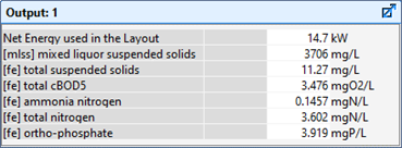
Figure 18‑5 – Unoptimized Outputs of a 0-Day Steady State Simulation
Preform DDO on 0-Day Simulation
13. A Python script has already been created for use in this tutorial. Locate and open the Python script called ‘tutorial-18-0Day.py’. The Python script can be found in the following directory:
\layouts\08tutorials\
14. Save the Python Script. Save the script in the current working directory.
15. Add the Script to GPS-X. Open the Python Script Manager in GPS-X and add the Python script to GPS-X.
16. Edit the Script. Press the Edit button to open the script in Notepad. We will now explore what the script is doing:
The ctypes Python library is used to interface the DDO and sobol_sampling functions found in the ddo Dynamic Link Library (DLL) within the GPS-X instillation. Using the ctypes library, the input types of the ddo function have been defined using the data types available in the ctypes library.
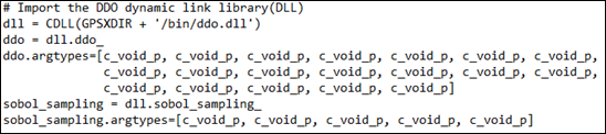
Figure 18‑6 - Adding the Dynamic Link Library Functions to the Python Script
Next, we define the optimization conditions to be used in the optimization:
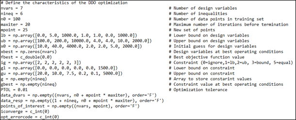
Figure 18‑7 – Optimization Problem Definition
· nvars – represents the number of target variables to be manipulated in the optimization. This is the number of inputs we will be changing in GPS-X
· nineq – represents the number of constraints in the optimization problem
· n0 – This is the number of points that will be used in the training set
· maxiter – This is the maximum number of optimizer iterations that can occur before the optimization is terminated
· mpoint – This is the number of points that will be looked at in each optimization iteration
· lb – These are the lower bounds of the design variables
· ub – These are the upper bounds of the design variables
· x0 – These are the initial guesses to be used for the design variables
· xbest – This is a list that contains the design variable values that resulted in the best objective function value
· fbest – This variable contains the best objective function value
· gl – This is the lower bound of the constraints
· gu – This is the upper bound of the constraints
· ig – This represents the type of constraint that is being used. 0 indicates that the constraint can be ignored, 1 indicates that the constraint is a one-sided greater than or equal to constraint, 2 indicates that the constraint is a one-sided less than or equal to constraint, 3 indicates that it is a two-sided constraint, 5 represents that it is an equality constraint
· g – This is a list where the current values of the constrained variables are stored
· gbest – This is a list that contains the value of the constrained variables when using the design variables that resulted in the best objective function value
· data_dvars – A matrix that is used to contain the manipulated points to be tested
· data_resp – A matrix that contains the results of the tested conditions
· points_of_interest – Is a matrix of points that the ddo optimizer would like to investigate
· PTOL –Is the optimizer tolerance to be used for termination prior to reaching the maximum number of iterations
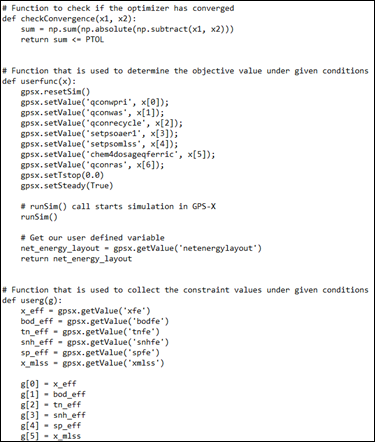
Figure 18‑8 - Functions to Set Input Values and Collect Outputs
The checkConvergence function is used to check if the change in design variables used by the optimizer is less than the defined tolerance, indicating the optimizer has converged on a solution.
The userfunc function resets the simulation so all simulations start from the same point and sets the current values of the design variables in GPS-X. After setting these values, the GPS-X simulation is run. The value of the objective function is collected at the end of the simulation and returned from the function.
The userg function collects the value of the constrained variables at the end of the 0-Day simulation.
The remaining code in the Python script is responsible for running the DDO algorithm and displaying feedback about the progression of the DDO algorithm. It can remain unchanged in your DDO applications
17. Run the Script. Press the Run Script button with the script highlighted. The script will require a few minutes to run. Note that the time required to run the script will be dependent on the speed of your workstation and the complexity of the model.
After the simulation has been run, the Python script manager will display the best value of the objective function value it found, the design variable settings used to obtain that objective function and the values of the constraints under those conditions. The results of the 0-Day DDO optimization can be seen in Figure 18‑9.
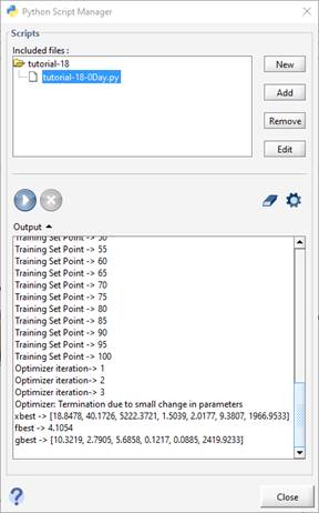
Figure 18‑9 - Results of the 0-Day DDO Optimization
Note: When using the DDO optimizer, ensure that you verify that a solution has been found that satisfies all of the defined constraints. The optimizer will attempt to meet all constraints, but if the system is over constrained, it will provide a solution that exceeds the definition constraints. You will not be warned by the optimizer if a constraint has been exceeded.
18. Modify the Python Script. Change the value of n0 to 15, the value of maxiter to 5 and the value of mpoint to 7.
19. Save the Python Script.
20. Run the Script. This will illustrate the tradeoff between computational speed and optimizer performance that is faced when choosing the number of iterations that the optimizer will use. By decreasing the number of iterations used, a feasible solution is obtained in less computational time, but our objective function has increased by approximately 0.5 kW. It is important to consider this tradeoff when constructing an optimization problem
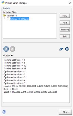
Figure 18‑10 - Results of the Modified 0-Day DDO Optimization
Preform DDO on Dynamic Simulations
While optimizing plant operation in a 0-Day simulation can help identify possible operational improvements, it only provides a snapshot of the actual plant operation. By preforming a dynamic simulation, you can determine parameter settings that are optimal over long periods of standard operating conditions or during extreme weather conditions. Python and GPS-X both allow you to insert real plant data into the simulation, allowing you to perform an optimization on real operating conditions experienced at your plant.
Note: When preforming DDO on Dynamic Data, the process can be very lengthy. The simulations in this section may take multiple hours to converge to a solution depending on the speed of your workstation.
21. A Python script has already been created for use with this section of the tutorial. Locate and open the Python script titled ‘tutorial-18-Dynamic.py’. The Python script can be found in the following directory:
\layouts\08tutorials\
22. Save the Python Script. Save the script in the current working directory
23. Add the Script to GPS-X. Open the Python Script Manager in GPS-X and add the Python script to GPS-X.
24. Edit the Script. Press the Edit button to open the script in Notepad. We will now discuss what has been changed from the ‘tutorial-18-0Day.py’ script:
The script has been modified to run a 1.0-day dynamic simulation. Due to the simulation being changed to a dynamic simulation, a communication interval will now occur in the simulation. A function, as seen in Figure 18‑11, will be called at each communication interval to collect the current value of the objection function variable and the constraints and add it to the cumulative sum. We will be minimizing the total net energy usage over the simulation period in this example.
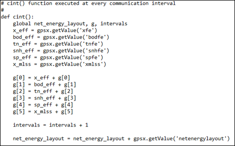
Figure 18‑11 - Function called at each Communication Interval in the Simulation
In this example, all of the collected constraint values are expected to exceed the bounds set in the 0-Day simulation as cumulative sums are now being collected rather than an instantaneous value. To accommodate this, we will constrain the average value of each constraint experienced across all simulated communication intervals. This is done by creating a variable which will track the number of communication intervals experienced during the simulation and dividing each element in array g by it. The code used to perform this average can be seen in Figure 18‑12.
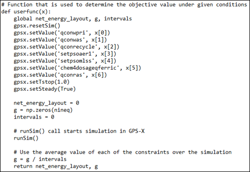
Figure 18‑12 - Updated userfunc Function that Averages the Constraint Values Collected in g
25. Create an Input controller for the Influent Flow type. This variable is accessed by right clicking on the Influent Object and going to Flow > FlowData.
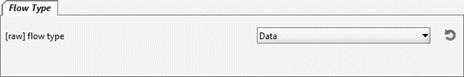
Figure 18‑13 - Influent Flow Type Controller
26. Using the input controller, set the influent flow type to Diurnal Flow.
27. Run the Optimization Script.
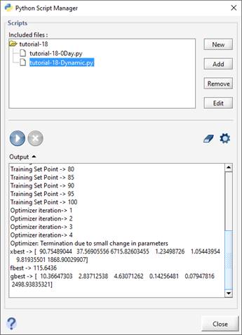
Figure 18‑14 - DDO Optimizer Output for a 1-Day Dynamic Simulation with Diurnal Influent Flow
28. After the simulation has finished, change the influent flow type to Sinusoidal and run the Script again. This will allow you to see the effects it has on the optimization results.

Figure 18‑15 - DDO Optimizer Output for a 1-Day Dynamic Simulation with Sinusoidal Influent Flow