Tutorial 10
Problem Statement
Model calibration and verification is one of the most important components of any modeling project. Model calibration, also known as parameter estimation, is defined as the process of adjusting model parameters such that the difference between observed and simulated results is minimized. For example, if the difference between observed and simulated effluent suspended solids is too large, it is likely that you will want to adjust some of the model parameters.
GPS-X provides a very convenient way of adjusting the model parameters, based on a non-linear dynamic multi-parameter optimization algorithm (Nelder-Mead simplex method).
In this example, the estimation of two kinetic parameters (heterotrophic growth rate and half saturation constant) is carried out in order to fit the model-predicted soluble substrate concentration with the measured data. Although this is a simple example, using only a CSTR unit process, the procedure outlined below is the important subject.
Objectives
The purpose of this tutorial is to develop a basic understanding of parameter estimation using GPS-X. After this tutorial, you will be able to target variables that you are interested in fitting to the data, select the model variables to be adjusted and specify the form of the objective function. Other optimizer variables such as termination criteria and number of data points will be explained in this tutorial.
Initial Manual Calibration
1. Start a new layout.
2. Switch to the Carbon, Nitrogen (cnlib) library.
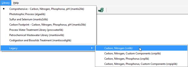
Figure 10‑1 – Switch Library to cnlib
3. Drop a single Completely-Mixed Tank on the drawing board. Confirm that the process model is mantis. The stream labels will be left at their defaults (should be the numbers 1 to 4).
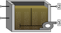
Figure 10‑2 – Simple Layout for Optimization
4. Set the tank’s initial conditions. For this example, we will just access Initial Conditions > Initial Concentrations and change initial readily biodegradable substrate to 200 mgCOD/L.
5. Change the tank’s parameters.
· Set Input Parameters > Operational > specify oxygen transfer by… to Entering Airflow.
· Set the air flow into aeration tank to 40,000 m3/d.
|
|
6. Change the simulation setup parameters. Open the Site Properties window by clicking on the button in the upper left corner of the drawing board. Open the Simulation Setup tab. |
Change the stopping time to 0.25 days, and the communication interval to 0.01 days.
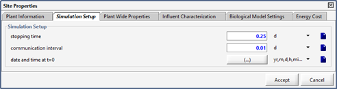
Figure 10‑3 – Changing Simulation Setup
7. Save the layout with the name ‘tutorial-10’.
8. Switch to Simulation Mode.
9. Create a graph. Add readily degradable soluble substrate (from Output Variables > Concentrations > Organic Variables > More…) on a graph and change the limits to 0-300 mgCOD/L.
10. Run a 0.25-day simulation (make sure Steady State is NOT checked). Your output should match that of the graph in Figure 10‑4.
Figure 10‑4 – Readily Degradable Substrate Output Graph
You will now optimize two kinetic parameters in order to obtain the best fit between effluent soluble substrate data and simulation results.
11. Create input controls. Place the following parameters (found in the tank’s Input Parameters > Kinetic) on an input control tab:
· heterotrophic maximum specific growth rate
· readily biodegradable substrate half saturation coefficient
Set limits of 0.5-5 d-1 for the growth rate, and 0.5-10 mg COD/L for the half saturation coefficient.
12. Add observed data file. Create a spreadsheet file with the example data listed in Table 10‑1. Save it in the same directory as your layout file, then add it to that layout. If you need a reminder of the process, see Tutorial 6.
Table 10‑1 – Example Data for Optimization
|
t |
ss2 |
|
d |
mgCOD/L |
|
0.00 |
213.5401 |
|
0.01 |
209.4151 |
|
0.02 |
197.8075 |
|
0.03 |
187.389 |
|
0.04 |
172.1104 |
|
0.05 |
185.44 |
|
0.06 |
178.8617 |
|
0.07 |
148.0012 |
|
0.08 |
152.297 |
|
0.09 |
142.1657 |
|
0.10 |
120.4514 |
|
0.11 |
117.4068 |
|
0.12 |
120.551 |
|
0.13 |
95.89756 |
|
0.14 |
84.38476 |
|
0.15 |
79.90364 |
|
0.16 |
73.47583 |
|
0.17 |
47.58231 |
|
0.18 |
39.27833 |
|
0.19 |
28.0756 |
|
0.20 |
16.67731 |
|
0.21 |
4.3656 |
|
0.22 |
0.624523 |
|
0.23 |
1.157525 |
|
0.24 |
0.985331 |
|
0.25 |
1.235542 |
13. Save the layout.
14. Re-run the simulation. Manually change the growth rate and half saturation parameters with the goal of minimizing the difference between the simulated and measured data. Figure 10‑5 displays the initial graphical output prior to making manual changes to the growth rate and half saturation parameters.
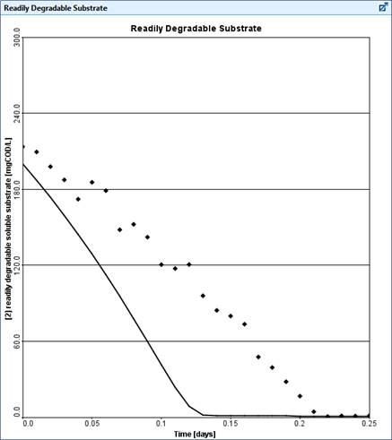
Figure 10‑5 – Readily Biodegradable Substrate Output Graph with Example Data
Automatic Calibration Using the Optimizer
After manually calibrating the model in the previous section (i.e. adjusting the heterotrophic maximum specific growth rate and readily biodegradable substrate half saturation coefficientparameters using the sliders and re-running the simulation), you will now set up the automatic parameter optimization tool to perform a search routine to find the best set of parameter values to fit the prediction to the measured data.
|
NOTE: It is always advisable to carry out a manual calibration first to determine the effects of parameters on the simulated response before carrying out an optimization. |
15. Switch to Modelling Mode.
|
|
16. Click on the Optimize button on the top toolbar and select Optimize Setup. This will display the Optimizer Setup Wizard. |
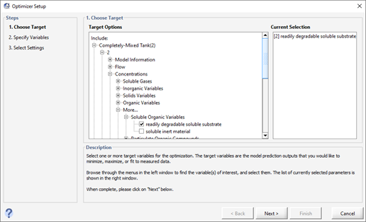
Figure 10‑6 – Optimize Setup Wizard (Target Variables)
17. Select the Target Variable. In this case, it is the readily degradable substrate in the reactor. It can be found under:
Completely-Mixed Tank(2) > 2 > Concentrations > More… > Soluble Organic Variables
18. Click Next to proceed to the next stage.
19. Select the Optimize Variables. These are the input parameters being adjusted during the fitting exercise. Select the following variables:
· heterotrophic maximum specific growth rate
· readily biodegradable substrate half saturation coefficient
These can be found under:
Completely-Mixed Tank(2) > Kinetic > Active Heterotrophic Biomass
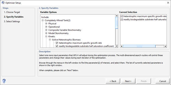
Figure 10‑7 – Optimize Setup Wizard (Optimize Variables)
20. Click Next to proceed to the next stage.
21. Specify Optimizer Settings. The last step in the process is to specify which kind of optimization we are doing. We will use Fit to Data, Time Series, and Maximum Likelihood.
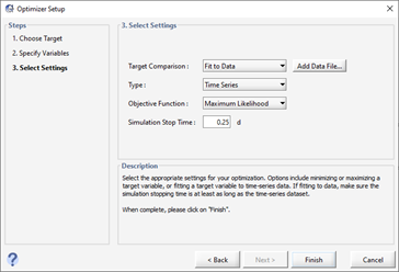
Figure 10‑8 – Optimize Setup Wizard (Optimizer Settings)
We can also use the “Add Data File…” button here to add data if needed, but we have already specified our data file earlier (step 12) so we do not need to do it again here.
22. Click Finish to complete the set up. Switch to Simulation mode.
Note that a new Input panel has been created with our two Optimization parameters already set to optimize mode. The target variable is also now plotted on a new graph. (These two actions may leave you with tabs with nothing in them. Feel free to delete them).
|
|
23. Enter Optimization Mode. Press the Optimize button on the main toolbar and select Optimize Mode. When optimize mode is active, the optimize icon on the main toolbar will change to display a green checkmark. |
24. Save the layout.
25. Start the simulation. GPS-X will automatically perform a number of simulations in a row, adjusting the values of the two optimize parameters each time to get a better fit to the observed data. Once the simulator has determined that no better fit can be achieved, it will stop. This should only take a few seconds.
At each optimization iteration, GPS-X plots the simulation results (i.e. predicted values) that correspond to the current parameter values. It retains the 7 most recent simulations on the graph. You can change the number of run curves on the graph by going to View > Preferences > Input/Output > Number of runs displayed (analyze/optimize). The simulation results are shown by a black line and the data are shown by red markers.
A plot of the fitted model and the measured data is shown below.
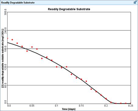
Figure 10‑9 – Results of
Optimization
Note that the initial parameter values used in the optimization are the default values found in GPS-X. After running an optimization, a Solution Report is generated for the optimization in the Command Window. Open the Command Window by pressing the Simulation Control button on the simulation toolbar and selecting the Command Window option or by right clicking on the area next to the output tabs and selecting Command Window. The Solution Report contains the results of the statistical analysis and the final parameter values. The Solution Report can be seen in Figure 10‑10.
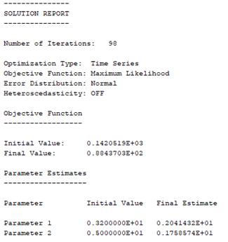
Figure 10‑10 - Optimization Solution Report