Tutorial 5

Influent Data & Influent Advisor

Problem Statement

You have some historical data related to the influent wastewater for your plant and it does not resemble the default data presented in the GPS-X influent object forms.  Unfortunately, a full characterization of your influent wastewater has not been performed.  Nevertheless, you need to estimate the influent wastewater characterization so that the model can be used with an influent that approximates your influent data. 

Objectives

In this tutorial, you will investigate the influent models, the impact of the local biological model on the influent calculations and the use of Influent Advisor as a tool to help characterize influent data.

Influent Data

The following historical data have been gathered at your plant and represent average values for your influent.

Table 5‑1 – Average Historical Data

Measured Parameter	Value	Units
total COD	365	gCOD/m^3
ammonia nitrogen	26	gN/m^3
total TKN	36	gN/m^3
total carbonaceous BOD5	190	gO2/m^3
soluble COD	68	gCOD/m^3
total suspended solids	210	g/m^3
volatile suspended solids	168	g/m^3
soluble TKN	31	gN/m^3

1. Create a New Layout.  Press the New button on the main toolbar.

2. Select a library.  In this tutorial, we will be using the Comprehensive – Carbon, Nitrogen, Phosphorus, pH (mantis2lib) library.  If it is not already selected, choose it from the ‘Library’ menu.

3. Place an influent object on the drawing board.  From the Influent group in the Process Table, drag a Wastewater Influent object on the drawing board.

4. Save the layout as `tutorial-5’.

5. Switch to Simulation Mode. We will be using a scenario to demonstrate the changes for this case study.

6. Create a new scenario named Influent. This process is described in Tutorial 3 in the                                                 Using Scenarios section.

7. Open the Influent Advisor tool.  To do this, right-click on the influent object and select Composition > Influent Characterization.

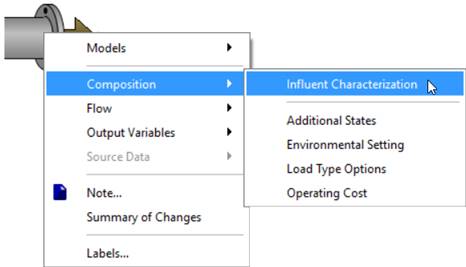
Figure 5‑1 - Accessing Influent Advisor Tool

8. Adjust values under “User Inputs”.  You will notice that under the “User Inputs” section of the Influent Advisor tool are various values that you can change.  From our list of data in Table 5‑1, only the first three values are immediately accessible.

9. Enter the values for total COD, total TKN, and ammonia nitrogen. Press Accept. In Figure 5-2, the entries are shown in green, indicating that these changes are part of the Influent scenario you created earlier.

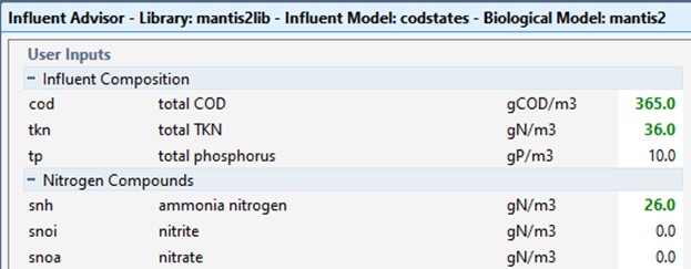
Figure 5‑2 – Adjusted Values

10. Check the remaining data in the table against their corresponding values in the Influent Advisor.  You will find the remaining variables in the right-most column (Composite Variables). 

The values reflect the new COD, TKN and ammonia input, but use the default influent fractionation. 

Note that the plant data differs from the calculated values displayed in the Influent Advisor tool.

Table 5‑2 - Plant Data vs Calculated Data

Parameter	Plant Value		Displayed Value		Units
total COD	365	-		gCOD/m^3
ammonia nitrogen	26	-		gN/m^3
total TKN	36	-		gN/m^3
total carbonaceous BOD5	190	188.2		gO2/m^3
soluble COD	68	125.2		gCOD/m^3
total suspended solids	210	185.3		g/m^3
volatile suspended solids	168	139.0		g/m^3
soluble TKN	31	28.9		gN/m^3

Clearly, the influent model calculations are inconsistent with the data for your plant indicating that one or more of the default settings (i.e. composition data or stoichiometric fraction) are inconsistent with your wastewater. 

In the next section, we will investigate the steps required to reconcile these discrepancies.

Using Influent Advisor

The Influent Advisor tool has been designed to make the characterization of the influent waste stream as straightforward as possible.  It would be possible to run a series of simulations (while adjusting influent parameters on sliders and observing plotted outputs) to find the correct settings, however this method would require setting up input controllers and output tables/graphs and could be potentially time-consuming.

The Influent Advisor tool shows all input and output in an interactive way, allowing users to determine which inputs affect each output, and to trace all dependencies.  The window contains three columns:

· User Inputs

· State Variables

· Composite Variables

We will now browse the various calculations and variables that make up our desired data.

11. Find the VSS variable in the Composite Variables column and click on the value. The VSS row will be highlighted and if you scroll up and down the page, you will also notice that several other rows have been highlighted in a lighter blue color. These are the variables that are used to calculate the VSS value.

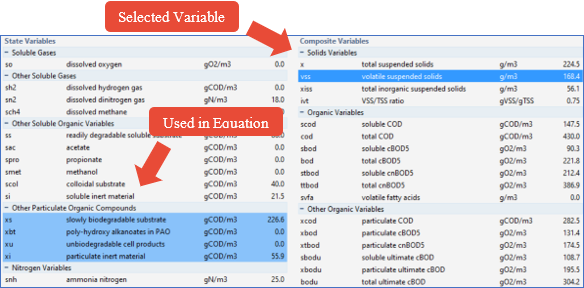
Figure 5‑3 – Influent Advisor showing Variable Relationships

Right at the bottom of the tool (scroll down), the actual formula is displayed (see Figure 5‑4).  This formula corresponds to the formula used in GPS-X to calculate the value clicked on, in this case vss.

Figure 5‑4 – Equation for VSS

Let’s proceed to adjust the influent parameters (fractions and/or concentrations) to reconcile the model predictions with the measured values.

12. Note that a particulate VSS to TSS ratio is used in the calculation of TSS. Select total suspended solids (x) from the Composite Variables table. This is one of several important relationships that can be calculated from the existing data.  For instance:

VSS:TSS ratio (ivt) = 168/210 = 0.8

13. Enter this value into the User Inputs column under the Influent Fractions sub‑heading.  Note that doing this seemingly results in values further away from what you are looking for.  Further changes will be required.

14. Click on VSS to display the calculation formula.  By continuing to click on the cells in the formula, you should be able to determine that vss is a function of the Particulate Organic Compounds, such as xi (particulate inert material), xu (unbiodegradable cell products), and xs (slowly biodegradable substrate).  The VSS is lower than our target, meaning that we must distribute more of the influent COD to the particulate forms (and less to the soluble forms).

15. Adjust the stoichiometric ratios in the Organic Fractions sub-heading to increase the particulate COD concentrations.  Try the following changes:

· set soluble inert fraction of total COD to 0.02,

· set readily biodegradable fraction of total COD to 0.15, and

· set colloidal fraction of slowly biodegradable COD to 0.05.

These changes force more of the COD into the xs (slowly biodegradable substrate) state variable, which therefore increases VSS and TSS.

16. Lastly, adjust the soluble TKN (stkn) value under the Composite Variables > Nitrogen Concentrations Headings.  Click on the equation to determine the appropriate input parameter(s) to adjust and make the necessary change(s).  You may find that adjusting the nitrogen variables causes the TSS to change.  Make further adjustments to the influent COD fractions to bring the TSS back to the target.

NOTE: In reality, you will characterize your influent and adjust these unknown parameters based on the model behavior and how that model behavior relates to what has been observed or measured at the plant.  Each wastewater is different, and each will require some adjustment of these parameters to get a characterization that results in model behavior that is consistent with your plant behavior.

An example of one possible solution to the influent characterization is shown in Figure 5‑5 and Table 5‑3 below.

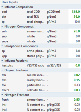
Figure 5‑5 - User Inputs

Table 5‑3 - Plant Data vs Entered Data with Calculated Results

Parameter	Plant Value	Entered Value	Shown Value	Units
total COD	365	365	-	gCOD/m^3
ammonia nitrogen	26	26	-	gN/m^3
total TKN	36	36	-	gN/m^3
total carbonaceous BOD5	190	-	188.5	gO2/m^3
soluble COD	68	-	69.7	gCOD/m^3
total suspended solids	210	-	209.7	g/m^3
volatile suspended solids	168	-	167.7	g/m^3
soluble TKN	31	-	30.6	gN/m^3
VSS/TSS ratio	-	0.8	-	gVSS/gTSS
soluble inert fraction of total COD	-	0.02	-	-
readily biodegradable fraction of total COD	-	0.15	-	-
colloidal fraction of slowly biodegradable COD	-	0.03	-	-
ammonium fraction of soluble TKN	-	0.85	-	-

17. Press Accept to save the changes to the influent advisor

Influent Advisor Warnings

Strictly as an exercise to demonstrate a point, you will now change the influent characterization so that a warning message is generated due to an improperly characterized influent.

18. Open the Influent Advisor tool, right-click on the influent object and select Composition > Influent Characterization.

19. Change the total TKN value (tkn) to 15 gN/m3 and hit ‘Enter’.

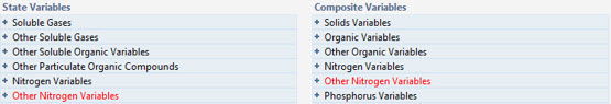
Figure 5‑6 - An Example of an Error in the Influent Advisor

You will notice that some state and composite variables have been highlighted in red. If a value in a collapsed menu is highlighted, that menu’s title will be highlighted red.  This indicates a negative value. These negative values can sometimes be the result of unusual or poor characterization data.  Negative influent concentrations can cause mass balance errors and convergence problems, so these values must be addressed before proceeding with a simulation. 

Note that if you attempt to Accept an improperly characterized influent, a pop up will be generated to warn you that the input values have resulted in negative state or composite variables, and you will not be unable to accept the characterization until this value has be addressed.

20. Change the total TKN value (tkn) back to 36 gN/m3 and hit ‘Enter’. 

Dynamic Data Validation

The Dynamic Data Validation tool is used to validate a dynamic input data set prior to using it to run a dynamic simulation. The tool will take the input data and preform influent characterization calculations at each time step in the data set, identifying any negative values.

21. Access the Dynamic Data Validation Tool. The Dynamic Data Validation tool can be found in the toolbar at the bottom of the Influent Advisor tool window.

Figure 5‑7 - Influent Advisor Toolbar

22. The Dynamic Data Validation Tool window will open and you will be required to add a pathway to both an input and an output data file.

There are two methods in which you can prepare the input file:

A. Manually prepare the spreadsheet outside of GPS-X and adding it directly to the Dynamic Data Validation Tool using the Browse button (Best used for multiple variables). Refer to Tutorial 6 for instructions on manually preparing spreadsheets.

B. Use the Create Template tool in GPS-X to automatically prepare the file (best for single variables).

This tutorial will focus on Method B.

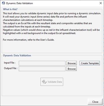
Figure 5‑8 - Dynamic Data Validation Window

23. Press the Create Template button.

24. Select the Parameters. GPS-X will prompt you to select the parameters you would like to include in the dynamic data validation.

Select the following parameters:

· cod / total COD

· tkn / total TKN

· snh / Ammonia Nitrogen

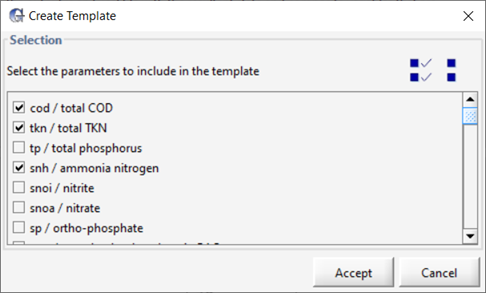
Figure 5‑9 - Dynamic Data Validation Parameter Selection

25. Save the file by pressing Accept. You will be prompted to save the Excel spreadsheet in the active directory using the same name as the layout. Press Save.

26. Open the file. GPS-X will prompt you to open the newly created spreadsheet. Press Yes.

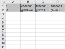
Figure 5‑10 - Excel Spreadsheet Generated by GPS-X

27. Enter the data found in Table 5‑4into the Input File. The bold red values in the table correspond to the poorly characterized values that will cause influent advisor to calculate a negative value.

Table 5‑4 - Data for Dynamic Data Validation

t	codcon1	tkncon1	snhcon1
d	gCOD/m3	gN/m3	gN/m3
0	370	36	25
1	375	36	40
2	374	37	25
3	376	38	26
4	373	40	29
5	378	42	28
6	380	15	28

28. Save the changes made to the Excel Spreadsheet.

29. Create an Output File. Press the Browse button next to the Output File entry field. You will be prompted to create an output file in the current working directory. Press Save.

30. Press Validate Data.

31. The results of the data validation will be recorded in the output file. After validating the data, GPS-X will prompt you to open the output file. Press Yes.

32. The Output File of the Dynamic Data Validation can be seen in Figure 5‑11.

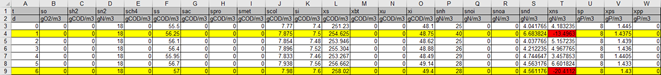
Figure 5‑11 - Output of the Dynamic Data Validation

Notice that row(s) 4 and 9 are highlighted yellow and contain cells that have been highlighted with a red background. The yellow rows indicate that the influent conditions used at this time step results in a negative value being calculated in the influent characterization. The red cells indicate the negative values calculated in the influent characterization

Previous Next