Parameters in process models are often not constant, but vary with time.
For example the oxygen mass transfer coefficient in an aerated tank is often slowly time varying.


GPS-XTM contains a suite of sophisticated tools allowing you to create advanced plant layouts, run interactive simulations, and perform in-depth analysis on model results.

PID Controller

ON/OFF Controller

Timer Controller

Flow Timer Controller

Scheduler Controller
In addition to stand-alone controllers, many unit processes have built-in PID controllers for easy setup (e.g. DO controller in aeration tank, RAS and WAS controller in secondary clarifier etc.).
A collection of standalone PID, PID feedforward, ON/OFF, Timer and Scheduler controllers allow you to build complex control systems like cascade ammonia based DO control, flow sequencing control in plant etc.
Evaluate
how changes in process and operating parameters affect various measures of plant performance

Determine
the relationship between the nitrification rate and temperature of the plant

Examine
how the MLSS concentration in the aeration tank affects the effluent ammonia concentration

Identify
the critical parameters for plant calibration
Determine the sensitivity of a nitrifying plant to wastewater temperature.
GPS-XTM performs successive steady-state simulations for a range of wastewater temperatures and plots the effluent ammonia as it is calculated.
Figure 1 shows effluent ammonia (Y-axis) as a function of wastewater temperature (X-axis).
From this graph, you can determine that some nitrification is begins to occur at around 7℃, and full nitrification is established at 20℃ and above.
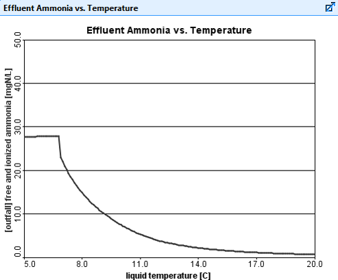
Figure 1. Automatic Steady-State Sensitivity Analysis of Effluent Ammonia vs. Wastewater Temperature
Determine the sensitivity of a nitrifying plant to wastewater temperature while experiencing a sinusoidal influent flow rate.
GPS-XTM runs a five-day dynamic simulation with a sinusoidal influent flow rate. This five-day run is repeated for a number of different wastewater temperatures (three in this example), and the results are plotted on the same output graph, as shown in Figure 2.
In this type of analysis, each line on the graph corresponds to the level of ammonia in the final effluent at a different wastewater temperature.
As displayed in Figure 2 there is increased nitrification occurring at higher influent temperatures. The concentration of effluent ammonia varies with time due to the sinusoidal influent flow rate.
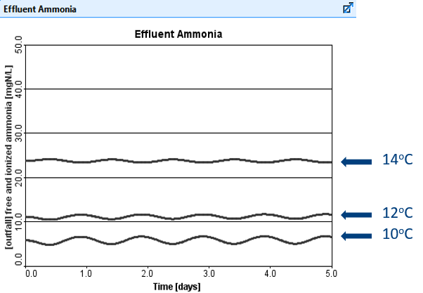
Figure 2. Automatic Sensitivity Analysis of Effluent Ammonia vs. Time (for three different temperatures)
Monte Carlo analysis in GPS-XTM allows users to generate probabilistic distribution of model outputs based on inputs with predefined probabilistic distribution. Both steady-state or dynamic Monte Carlo simulations can be performed in GPS-XTM. This analysis can be used to assess the effect of uncertainty in model parameter and or model input on the model outputs.
A robust Monte Carlo Analysis Tool allows users to evaluate plant performance when not all of the model inputs are well-known. Users can now run simulations using a typical distribution of values, rather than being forced to choose a single value, and observe a range of model outputs.
For example, users can predict a range of effluent ammonia concentrations given the typical range of nitrifier growth rates, even though the true actual growth rate isn't known.
The Monte Carlo Analysis Tool is a valuable addition to the GPS-XTM toolkit, and provides users with a way to bring the uncertainty of real life into their models.

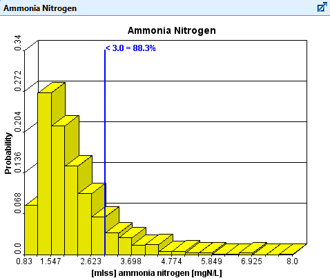
Monte Carlo Analysis Output for Effluent Ammonia Nitrogen

Model Calibration
Automatically find parameter values that minimize the difference between measured data and modeled results.

Process Control Optimization
Find the best design and process control parameter values.
GPS-XTM uses a robust multi-dimensional search routine that can easily handle multi-variable optimizations.
The objective is to determine the values of the heterotrophic maximum specific growth rate and the readily biodegradable substrate half saturation coefficient that allow for optimal matching to the diamond-shaped points on the graph displayed in Figure 1. These points are the results from a lab-scale bench experiment.
In this example the GPS-XTM optimizer is searching for the coefficient values that will minimize the difference between the simulated results and actual lab data.
The small diamond-shaped points represent the measured filtered COD, while the continuous lines are the simulated results of the batch experiment as GPS-XTM repeatedly searches for the appropriate coefficient values.

Figure 1. Kinetic parameter optimization showing successive guesses getting closer to the measured data points as the GPS-XTM optimizer automatically calibrates the model.
The optimized output is presented in Figure 2.
A similar calibration exercise using the optimizer can also be based on measurements from a full-scale wastewater treatment facility. For example, the optimizer could be used to find nitrifier growth rates using measured effluent ammonia data.
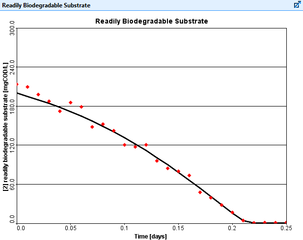
Figure 2. Optimized result fitting model output to measured data points.
The GPS-XTM Optimizer can be used to find appropriate control methods to minimize effluent concentrations from an activated sludge process.
The plant shown in Figure 3 is designed for biological nutrient removal. Under current operating conditions, this plant has an effluent total nitrogen (TN) of 10.0 mg/L.
In this example, the optimizer was used to vary the RAS flow, the WAS flow and the mixed-liquor internal recycle (MLIR) flow to meet a more stringent effluent TN objective of 7.0 mg/L.
The objective of this optimization is to minimize the effluent TN concentration by finding the best combination of the three flows, while ensuring that the maximum installed pumping capacities at the plant are not exceeded.
This optimization required 70 iterations to converge.
The table in Figure 4 shows the results of the optimization. The iteration number and the three optimized parameter values are shown along with the associated effluent TN concentration.
It can be seen from the results of this optimization that the plant can meet an effluent TN objective of 7.0 mg/L, if the current operating conditions are modified to the values determined by the GPS-XTM Optimizer.
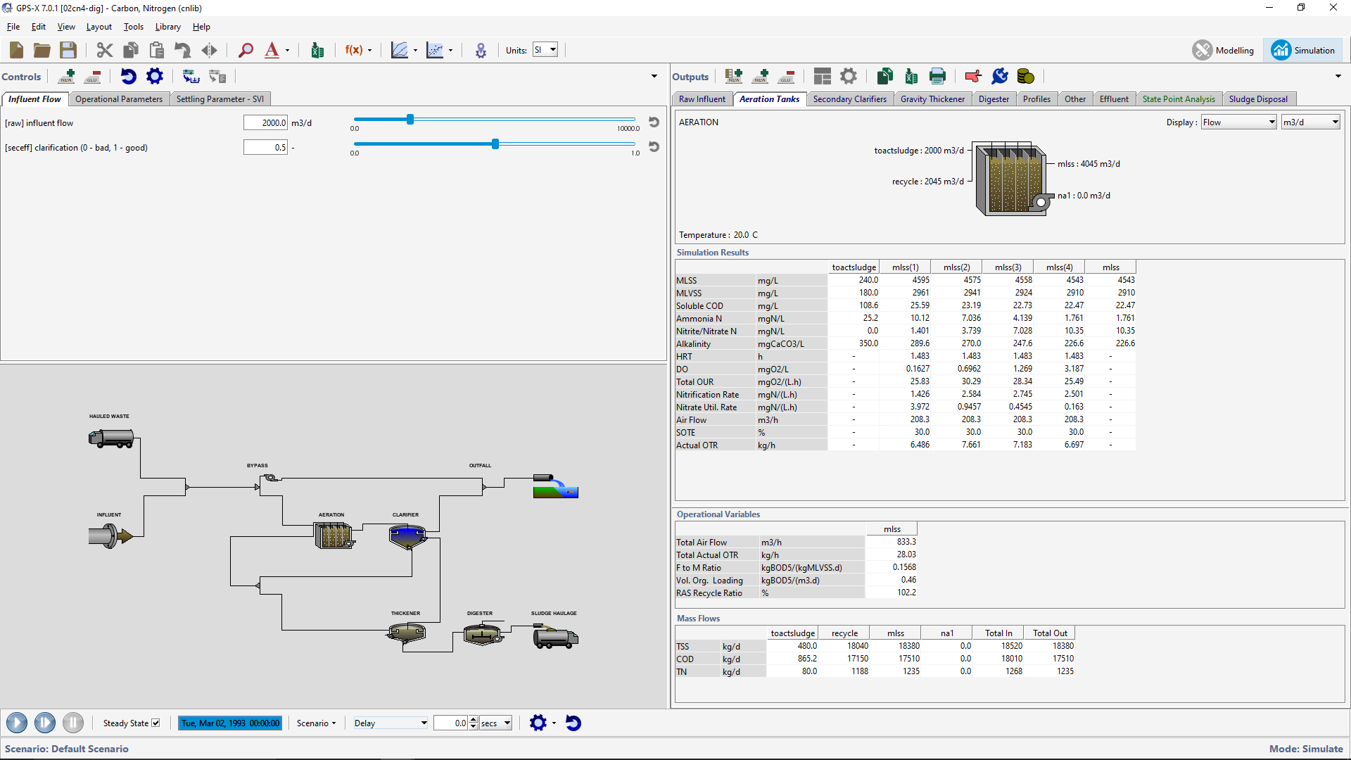
Figure 3. Example GPS-XTM layout for the process control optimizer runs.
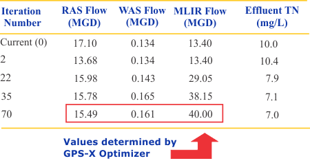
Figure 4. Optimized Process Control for Minimizing TN

Parameters in process models are often not constant, but vary with time.
For example the oxygen mass transfer coefficient in an aerated tank is often slowly time varying.

In these cases the model structure is likely to be incorrect. As a result, the model may only be able to represent the data well over short time intervals. In this case, using DPE will help compensate for the model error and allow acceptable fitting of the measured data.

If a model parameter is found to be relatively constant during normal process operation but is sensitive to process changes, you can track this parameter using the DPE feature and on-line data to help provide an early warning of process changes or upsets.
In GPS-XTM, dynamic parameter estimation is done by applying the time series optimization approach mentioned earlier to a moving time window. Instead of estimating parameters from an entire set of data, GPS-XTM calculates a set of parameter estimates for each time window using the parameter estimates from the previous time window as a starting guess. This approach can be used on a data file that is continually updated with new blocks of data or on a static file of time series data. Note that you can use any of the objective functions that are available for time series optimization when doing dynamic parameter estimation.
The length of the time window controls how often the parameters are updated. The shorter the time window, the more often the parameters are updated.
To improve the fit between the model results and data, a model parameter can be varied over the simulation period.
Typically the clarifier's flocculent zone settling parameter is set to one specific value over an entire calibration time period; this result is presented in Figure 1.
Holding this parameter constant does not result in the best fitting of the data, so this parameter can be varied with time to improve the agreement between the simulated model results and points on the graph, and to indicate the dynamic response of this parameter.
As presented in Figure 2, the flocculent zone settling parameter in the primary clarifier is adjusted at each 0.4-day time step to improve the fit of the model and actual data for the primary effluent TSS concentration presented in Figure 3.
Through comparison of Figure 1 and Figure 3, dynamically adjusting the flocculent zone settling parameter provides improved fitting to the data.
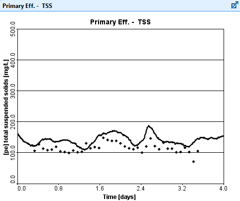
Figure 1. Simulation results for the primary effluent TSS concentration with a constant value for the clarifier Flocculent Zone Settling Parameter.
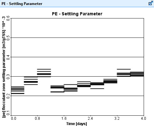
Figure 2. Values of the Flocculent Zone Settling Parameter over the simulation time period.
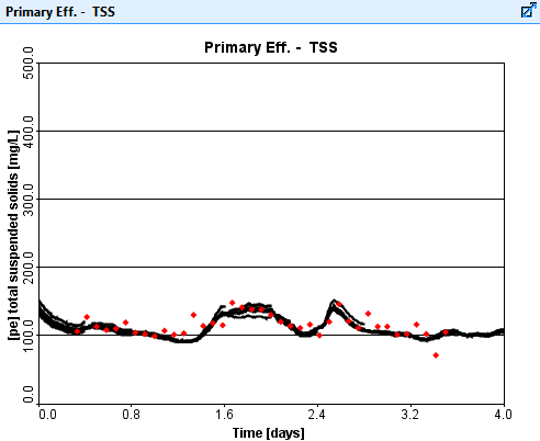
Figure 3. DPE results for the primary effluent TSS concentration.
Wastewater plants are variable, and it can be difficult to create a simulation tool that can handle all possible layouts and desired variables. Taking advantage of the customizability available in GPS-XTM users can generate input and output variables and use them as if they were part of the original layout.
Figure 1 presents a graph of the influent flow and the oxygen uptake rate.
New input and output variables are created by the user using the ACLS language. GPS-XTM incorporates these variables into the user-defined input and output menus, so in this particular instance they can be used as input controllers or added to an output graph.
Figure 2 presents the same graph as in Figure 1 but with the addition of the user defined variable for the oxygen uptake rate with added noise.
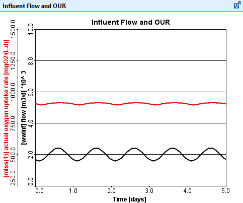
Figure 1. Influent Flow Rate and Actual Oxygen Uptake Rate vs. Time.
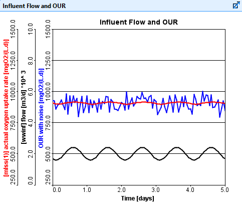
Figure 2. Influent Flow Rate, Actual Oxygen Uptake Rate, and Oxygen Uptake Rate With Noise vs. Time.
We have developed an integrated interface for creating and executing python scripts from within GPS-XTM. The python script can interact with GPS-XTM models to exchange data and allow you to incorporate supplemental analytics on the model data.
By allowing custom scripts to be run in GPS-XTM, you can use all of the tools available in python to extend what is possible in GPS-XTM. While the applications of GPS-XTM are diverse, it may not always be built generally enough to provide the exact analysis or data visualization options you would like for your project.
By using python, you can do things such as create custom plots, introduce new types of statistical analysis and automate repetitive tasks in ways that are not possible using only GPS-XTM.


While you can use python to fit a 3rd party component into GPS-XTM, you can also use python to integrate the GPS-XTM model as a component of your bigger enterprise software.
Using the GPS-XTM Model-as-a-Service and python, you can programmatically run and extract results from a model directly from your own software solutions.
GPS-XTM may be the puzzle piece that you've been searching for.

Add New
Add new rates (rows in the matrix) or involve additional states (columns in the matrix)

Change Existing
Change kinetic equations or stoichiometric relationships

Modify Values
Modify default values of various parameters

Implement Types
Implement new biomass or substrate types

Inhibit
Inhibition of growth in the presence of toxic substance

Create Processes
Create additional transformation processes that operate independently of existing ones
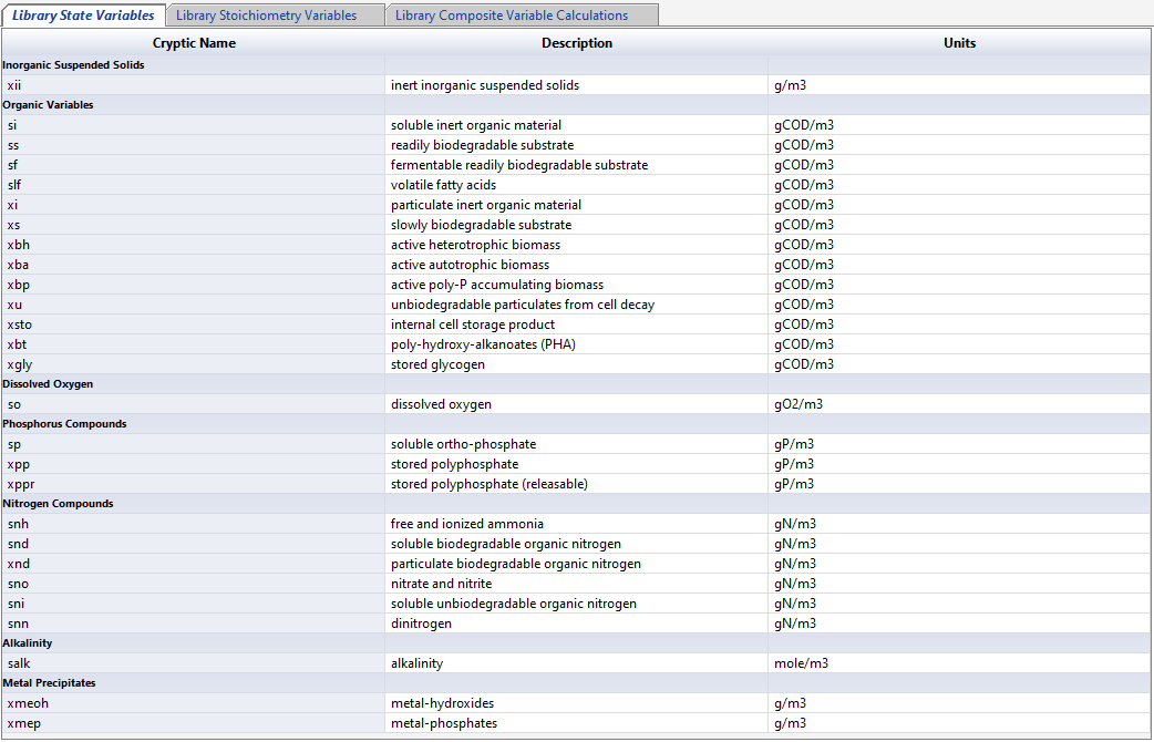
Access a summary of the state, stoichiometric, and composite variables.
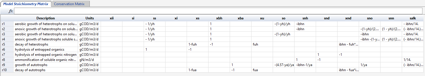
View and make edits to the model stoichiometry and conversation matrices.
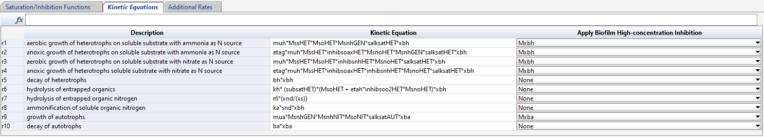
Access and make edits to various kinetic and rate equations.
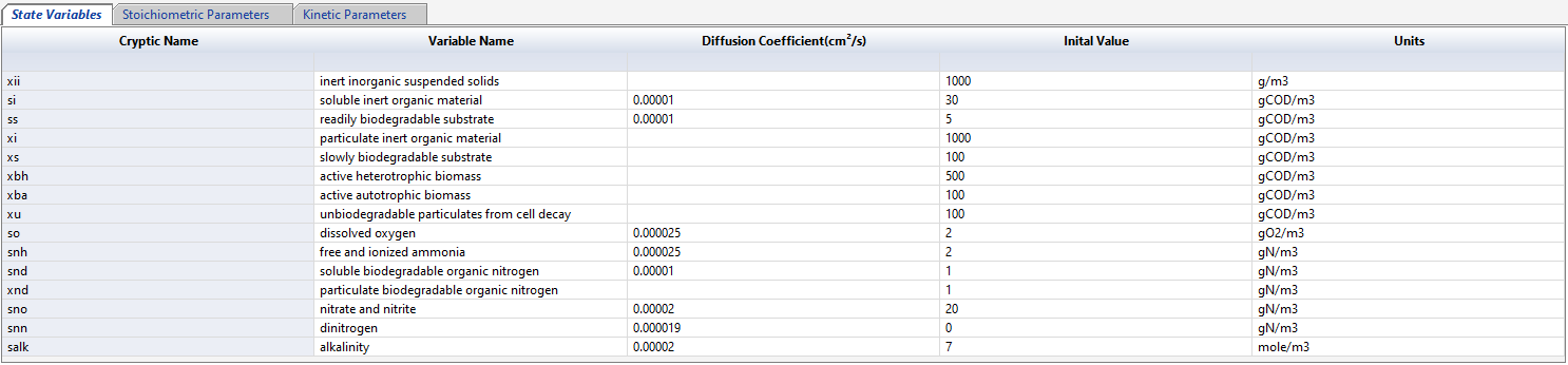
Access and make edits to the model state variables, stoichiometric parameters and kinetic parameters.
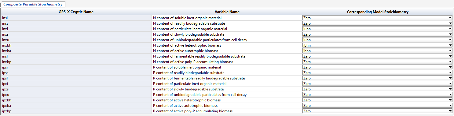
Select the model stoichiometry for the composite variables.