Tutorial 3
Editing Layouts and Using Scenarios
Problem Statement
For this tutorial, consider a situation where the plant you developed in the first tutorial is expected to treat increased flow due, for example, to extra sewer connections. Assume that the plant has adequate aeration capacity but requires an extra clarifier.
Objectives
GPS-X makes it easy to build models to help you examine changes in plant design and operation. This tutorial will show you how to use the layout editing tools such as Copyand Paste to make additions to the layout. Once the new model is built, the scenario features of GPS-X will be introduced. Using scenarios, you can set up specialized data sets for comparing the performance of the clarifiers in the event of uneven flow distribution under both steady state and dynamic conditions.
When you are
finished with this tutorial, you will have developed the ability to
create and edit plant layouts and will have developed a better
understanding of static[3]
data input and output in GPS-X. You will be able to prepare
simulation scenarios to test different hypothetical situations and
be able to run the scenarios to test alternative plant designs or
examine operational changes.
Expanding the Plant
1. Open the layout built in Tutorial 1 and save it as ‘tutorial-3’ using File > Save As...
2. Switch to Modelling Mode (if not already there) using the button on the top right-hand side of the screen.
3. Display the grid on the drawing board. Select View > Display Grid from the main menu.
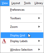
Figure 3‑1 - Selecting Display Grid
4. Display a larger drawing area. In order to expand on the layout, more space is required on the drawing board. Open the Locator window under View > Zoom > Locator and outline a larger working area. Alternatively, the mouse wheel can be used to scroll out and the desired work area can be highlighted and then zoomed in on by using the Zoom to selection/plant button. This will allow you to place more objects on the drawing board. More details regarding use of the Locator are presented in Tutorial 1.
5. Move the influent and plug-flow tank objects by clicking and dragging out a box around the influent and plug-flow objects. Then, with the mouse button pressed on one of the selected objects, drag the selected area to its new location on the drawing board (see Figure 3‑2).
6. Move the wastewater outfall object by clicking and dragging the object to the right.
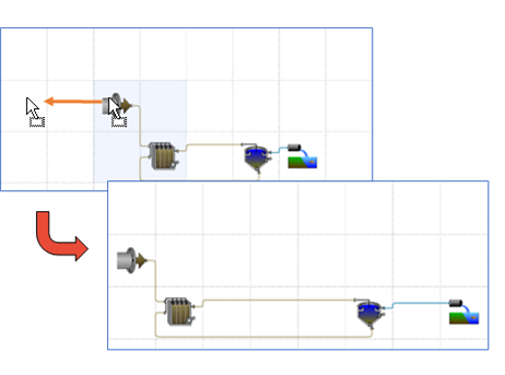
Figure 3‑2 – Moving Multiple Unit Processes
7. Copy the final clarifier. First, select the existing secondary clarifier located on the drawing board. The clarifier grid cell will show a light blue background.
|
|
Click on the Copy button and then select a destination cell by dragging out a small box inside the destination cell. The destination cell will show a light blue background. |
|
|
Next, click on the Paste button. This will paste a copy of the clarifier and all its attributes to the new location. |
Your layout should now look like Figure 3‑3.
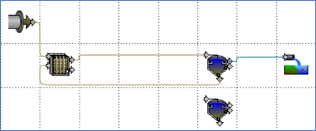
Figure 3‑3 - Copy/Pasted Clarifier
We will now complete the layout by adding the following:
· A two-way splitter to divide the mixed liquor from the aeration tank to the two clarifiers
· A two-way combiner to join the recycled sludge from the two clarifiers with the raw sewage as feed to the aeration tank.
· A two-way combiner to mix the effluent overflow from the two final clarifier tanks
8. Delete unneeded connections. You can delete a connection by right clicking on the connection and selecting Delete Connection.
Alternatively, you can delete the flow lines by placing the cursor at the initiation or terminal point of a flow line and dragging the flow line to an empty space on the drawing board. As soon as the mouse button is released you will be prompted to confirm the deletion of the flow line.
Delete the connection from the plug flow reactor to the final tank, the connection between the clarifier underflow and the plug flow reactor and finally the connection between the clarifier effluent and the wastewater outfall.
9. Add processes to the drawing board. From the Flow Combiners and Splitters group in the Process Table we will need one 2-Flow Splitter and two 2-Flow Combiners. Position the objects so that your layout now resembles Figure 3‑4.
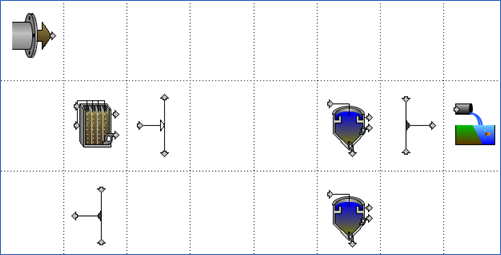
Figure 3‑4 - Add Splitter and Combiners
|
|
10. Flip the combiner below the Aeration Tank. To do this, select the combiner and press the Mirror button on the main toolbar. |
11. Connect all objects and label all units and streams. The last step of the plant expansion is to connect all the objects and label them appropriately as seen in Figure 3‑5 and described in Table 3‑1.
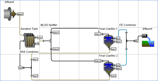
Figure 3‑5 - Processes and Streams Labelled Properly
|
NOTE: The colors of the flow lines each convey a specific meaning about the properties of the stream. Brown lines are used to represent the flows of wastewater. An example of this is your wastewater influent or the sludge leaving a clarifier Black lines are used to represent any streams where you are unable to tell what the outputs will be when the object is selected. An example of this is a combiner or splitter objects Blue lines are used to represent any flows of treated water. An example of this is the effluent stream leaving a clarifier overflow |
Table 3‑1 - Process and Stream Labels
|
Unit |
Label |
|
Wastewater Influent |
Label: Influent influent: wwinf |
|
Plug-Flow Tank |
Label: Aeration Tank overflow: mlss recycle: ras |
|
2-Flow Splitter |
Label: MLSS Splitter output#1: mlss1 output#2: mlss2 |
|
Circular Secondary Clarifier 1 |
Label: Final Clarifier 1 overflow: fe1 pump: was1 underflow: ras1 |
|
Circular Secondary Clarifier 2 |
Label: Final Clarifier 2 overflow: fe2 pump: was2 underflow: ras2 |
|
2-Flow Combiner for Recycled Sludge |
Label: RAS Combiner output: ras |
|
2-Flow Combiner for Final Effluent |
Label: FE Combiner output: fe |
|
Wastewater Outfall |
Label: Effluent |
12. Add a note to a process. Sometimes it is useful to make a note to remind yourself about certain details or reasons for changing something. These notes are just for your own reference and do not affect the simulation in any way.
Here, we will add a note to the Final Clarifier 2 unit. Right-click on it and chooseNote… from the popup menu. A blank window will appear in which description of the unit can be typed. Click Accept to close the Note window.
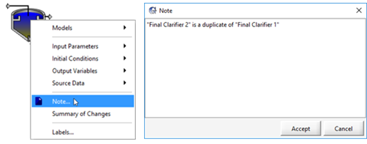
Figure 3‑6 – Add Note to a Process
13. Save the layout. Press the Save button on the main toolbar.
Using Scenarios
When organizing simulation runs it is useful to start with a base set of data, and then create one or more separate cases, which are modifications to the base data set. These cases are referred to as scenarios in GPS-X.
You can create any number of scenarios and in each scenario, you can specify the changes to the model parameter(s) which define that scenario. Those changes are saved so that they can be restored at any point in the future.
Creating and using scenarios is done in Simulation Mode.
In this section of the tutorial, we are going to use scenarios to investigate the effects of changing the following model parameters:
· Influent flow, to simulate the additional sewer connections
· Influent type, to simulate a dynamic fluctuation of the influent wastewater
14. Switch to Simulation Mode using the button at the top-right of the screen.
15. Create a new scenario by selecting Newfrom the Scenario menu on the Simulation Toolbar (at the bottom of the main window).
![]()
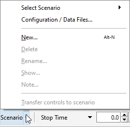
Figure 3‑7 - Create New Scenario
16. Type in a name for your new scenario (eg. “Expansion”) and Accept the form.
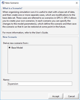
Figure 3‑8 – Name the Scenario
You will notice that the name of the active scenario is displayed under the Start button on the Simulation Toolbar.

Figure 3‑9 - Scenario Name Display
|
NOTE: You can change the active scenario by selecting it from the Scenario > Select Scenario list. The “Default Scenario” is the base case where all of the model parameters are set to the values defined when the model was built. If you return to modelling mode and make changes to the Default Scenario Parameters, these changes will be applied to all scenarios where that parameter has not already been specified. |
17. Add some parameter changes to the scenario. In this case, we will change the influent flow type and rate.
While remaining in Simulation Mode, access Flow > Flow Data from influent objects process data menu (ie. right-click on the object).
Change the flow type to Sinusoidal and change the influent flow to 5000 m3/d.
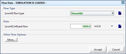
Figure 3‑10 - Changing Parameters in a Scenario
You will notice that changes made in a scenario are highlighted in green.
Accept the form.
18. If you do not already have an input controller (slider type) for the influent flow create one as described in the Creating Input Controlssection of Tutorial 2. Set the minimum and maximum values to 0 and 12,000 m3/d respectively.
19. Verify the parameter changes made in the scenario. Any changes made in a given scenario from the base scenario can be viewed by selecting Show on the Scenario menu on the Simulation Toolbar.
![]()
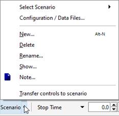
Figure 3‑11 - Show Changes Made to the Active Scenario
This window will show a summary of any variables that have been changed in the current scenario. The value that the variable was assigned when the model was built is shown in the grayed-out box. If any of the variables changed in this scenario appear on an input controller, an icon will appear next to the variable name to indicate the input controller.
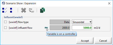
Figure 3‑12 - Summary of the Changes made in the Active Scenario.
|
|
Parameter changes in a given scenario can be directly edited in this menu by adjusting the setting of the box that is not grayed out. Additionally, any unwanted changes can be returned to their default value by checking the box next to the parameter name and pressing the Remove button in the toolbar. |
Accept the form.
20. Create an input control (slider type) for the split fraction (in the "MLSS Splitter"). Access this variable by going to Input Parameters > Splitter Setup. Set the minimum and maximum values to 0 and 1, respectively.
21. Create a horizontal bar chart for the solids profile in the new (copied) clarifier as described in the Analyzing the Plant section of Tutorial 2.
22. Create a X-Y graph for the effluent SS for each clarifier, and the combined effluent. In each case, the total suspended solids variable can be found in Output Variables > Concentrations of each object's outflow stream (i.e. right-click on the connection point, not the process itself). Display all three concentrations on one graph and rename the graphs appropriately. Set the minimum and maximum value to 0 and 120 mg/L respectively for each of the axis. Having the maximum locked, automatically change all of the values.
23. With the steady state box checked, run a 1-day dynamic simulation.
24. Change the split fraction to 0.3 using the interactive controller and increase the stop time to 2 days.
25. Resume the simulation using the Resume button (i.e. don’t restart it) and let the simulation proceed until it stops.
26. Increase the flow to the plant to 8,500 m3/d and increase the stop time to 3 days.
27. Resume the simulation.
A set of typical results are shown in Figure 3‑13. These graphs show the effect of the imbalanced flow split on final clarifier performance and combined final effluent SS.
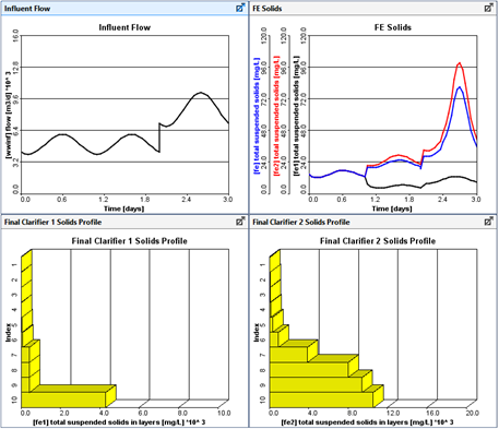
Figure 3‑13 - Typical Results