CHAPTER 9
Introduction
The Analyze module is used to conduct sensitivity analyses on your layouts. This module is an optional feature. If you have not purchased this module, contact us for pricing information.
The objective of a sensitivity analysis, in the context of simulation, is to determine the sensitivity of the simulation model's output variables (dependent variables) to changes in its parameters (independent variables). This provides insight into the model's behaviour and helps identify the parameters that have the greatest impact on the model. The results of a sensitivity analysis are very useful when setting up a parameter estimation run because they allow you to determine which parameters should be adjusted by the optimizer.
You can perform sensitivity analyses using any operational, stoichiometric, kinetic, or physical model parameter as the independent variable. In addition, you can conduct both steady-state and dynamic sensitivity analyses.
The material presented in CHAPTER 8 provides a basis for some of the discussions in this chapter. In particular, the material in the Steady-State and Dynamic Simulation sections will be needed to understand how to set up sensitivity analyses properly.
What is Steady-State Analysis?
Steady-State analysis is useful when it is unnecessary to introduce the extra complexity of dynamic changes. For example, graphs such as those in Figure 9‑1, which show the steady-state responses of model outputs to selected values of an input, might be sufficient for design purposes.
In operations, it is useful to know the ultimate or steady-state response of the plant, such as the effects of moving to a different operating point. A preliminary steady-state analysis may be sufficient to make useful predictions about the behaviour of the plant. It is important to keep in mind the proper interpretation of a steady-state analysis as described in the Steady-State Analysis section of CHAPTER 8. You can always enhance the analysis later by including a study of model dynamics.
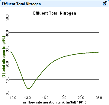
Figure 9‑1 – Example of Steady-State Sensitivity Analysis Graph
What is Dynamic Analysis?
When doing a dynamic sensitivity analysis there are two important cases to consider. In the first case the initial conditions are such that the process is initially at steady state. In the second case the initial conditions are dynamic. In CHAPTER 8, these two cases were examined with regard to the interpretation of the dynamic behavior that results. In general, you should assign initial conditions carefully. The same cautions apply when performing dynamic sensitivity analyses because here too you must specify appropriate initial conditions before running simulations with different values of the independent variable.
Examples of the two types of dynamic sensitivity analysis that you can perform are shown in Figure 9‑2.
In both cases, a dynamic simulation is run from time=0 until the Stop Time.
Panel A of Figure 9‑2 shows the change in dissolved oxygen (DO) concentration of the mixed liquor over time for several values of the wastage flow rate. Notice that the simulations all start at the same value, the preset initial value.
Now compare this to a similar sensitivity analysis setup shown in panel B. In panel B the simulations start at different values of DO since, in this type of analysis, the user has specified that the steady-state solver should be run before conducting the dynamic simulation.
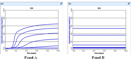
Figure 9‑2 – Dynamic Sensitivity Analysis (Steady-State Off vs On)
There are important differences in the interpretation to be given to these two cases. In the set-up resulting in the graph in Panel A of Figure 9‑2, the results demonstrate how the model responds to different values of the wastage rate starting from specific values of the model state variables, including the DO. In this case, it may be necessary to either extend the simulation or to perform a number of re-runs to observe the ultimate, periodic steady-state for the system. This type of analysis would be useful to answer questions such as the following:
· What is the dynamic response of the mixed liquor suspended solids concentration if the wastage rate is suddenly changed?
· How would the current DO concentration change over time if the air flow rate was suddenly turned up (or down)?
· What happens to the solids distribution over time if we quickly change to step feed operation in the plant?
In each case, there is an implied common starting point (current MLSS concentration, DO concentration or solids distribution) and a specified change in a model independent variable (wastage rate, air flow rate, or step feed). The immediate, short-term response of the model is of greatest interest.
In Panel B of Figure 9‑2, the situation is considerably different. In this case the simulation starts at a different DO value for each run. Here the steady-state solver is used to determine steady-state values for each value of the independent variable, set the initial conditions equal to these values and then started a dynamic simulation. The model is assumed to have been operating in a steady-state. At time=0 the value of the independent variable changes to that specified in the sensitivity analysis and a dynamic simulation is conducted until the specified stop time. This type of analysis is useful for answering questions such as the following:
· What variation in mixed liquor suspended solids can be expected over time for plant operation at different wastage rates?
· In the long run, how will the DO concentration vary over time for different values of the air flow rate?
· What is the solids inventory like if I use step feed all the time?
The common characteristic of these questions is the implied interest in long-term changes rather than the short-term effects of a sudden change. The initial value is not of concern; instead, it is preferred to avoid the situation where the model is making a transition from one periodic steady‑state to another and to examine the relative differences between these periodic steady‑states.
Time Dynamic and Phase Dynamic Analyses
The results of a dynamic sensitivity analysis can be displayed in one of two ways. Figure 9‑2 shows one way, that is, selected dependent variables plotted versus time. This is referred to as a time dynamic sensitivity analysis.
In some cases, it is desirable to view only the end-point of the dynamic simulation for each value of the independent variable. For example, you might want to ask:
· What is the value of the mixed liquor suspended solids one and a half (1 ½) days after a sudden change in the influent flow?
· What will be the value of the DO concentration at the end of each week when the plant is subject to a different, repeating diurnal flow pattern?
The questions suggest that the simulation result of interest is the value of the dependent variable at a specific point in time. This is referred to as a phase dynamic sensitivity analysis. Finding answers to these questions requires the ability to plot the values of dependent variables at the end of a simulation against the value of the independent variable. This type of plot, referred to as a phase diagram, is shown in Figure 9‑3.
There is one additional step to perform before initiating the analysis. A decision needs to be made whether the initial conditions are steady state or dynamic.
By selecting Steady-State (by checking it on the Simulation Toolbar) you direct GPS-X to calculate the steady-state values and use these as the initial conditions. If Steady-State is not selected, the manually entered initial conditions are used. These two types of analysis are referred to, respectively, as long and short-term analysis.
This difference is demonstrated in Figure 9‑3 which shows the same phase dynamic sensitivity analysis without steady-state initialization (Panel A) and with the initial conditions set using the steady-state solver (Panel B).
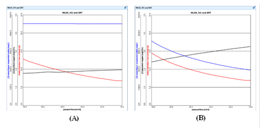
Figure 9‑3 - Phase Dynamic Sensitivity Analysis Graphs. (A) Starting from Non-Steady State. (B) Starting from Steady State
Steps in Sensitivity Analysis
NOTE: Sensitivity analyses are set up after the model has been built. The procedures in the remaining sections of this chapter assume that the outputs you want to display have already been set up and that the model which is the subject of the sensitivity analyses has been built.
After creating your layout, there are a few steps to set up a sensitivity analysis (steady-state or dynamic) as described below:
1. Switch to Simulation Mode.
2. Specify the model parameter to serve as the independent variable (see Creating A Control From An Independent Variable in CHAPTER 6).
3. Enter the minimum, maximum and increment value for the independent variable and set it as the appropriate analyze controller type (see Input Controls Properties in CHAPTER 6).
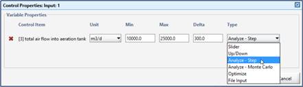
Figure 9‑4 – Set Input Control to Analyze Type
4. Select the desired type of analysis (steady-state, phase dynamic, time dynamic, monte carlo) from the drop-down list accessed through the Analyze button on the Main Toolbar or the Analyze menu item in the Tools Menu.
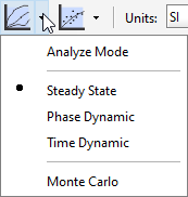
Figure 9‑5 – Accessing Analyze Features
5. Turn on Analyze Mode by clicking the Analyze button on the Main Toolbar (to toggle the mode) or accessing the Analyze menu item and selecting Analyze Mode. The status bar at the bottom of the main window will indicate that you are in Analyze Mode.
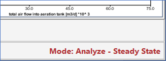
Figure 9‑6 – Status Bar showing Analyze Mode
6. Select the desired Stop Time (if applicable) and start the simulation.
Important Tips
1. There can be only one independent variable so do not specify more than one variable as an analyze type control. You can set up controls of other types and they will be displayed when you open the controls window. To avoid the effects of confounding variables, the other controls should not be changed when a sensitivity analysis is being performed.
2. Once the independent variable has been specified, the control is set to a non-interactive gauge; however, the program does not change to the analyze mode until the mode is changed manually to analyze.
As the independent variable is incremented, the analyze controller displays its current value in a non-interactive gauge as shown in Figure 9‑7. You can estimate the extent of completion by observing this gauge.
![]()
Figure 9‑7 – Analyze Controller
4. The outputs that are displayed when doing a dynamic analysis will depend on whether Time Dynamic or Phase Dynamic was selected from the Analyze menu. For Time Dynamic analyses, time is plotted on the X-axis, whereas for Phase Dynamic analyses, the specified independent variable is plotted on the X-axis.
What is Monte Carlo Analysis?
Monte Carlo analysis may be conducted as either a steady-state or dynamic analysis. The process for setting up a steady state or dynamic Monte Carlo analysis is similar to the set-up of the dynamic and steady state analyses outlined earlier in the chapter but there are a few differences which will be covered below.
Monte Carlo analysis functions in a similar way to the step analysis method discussed earlier in this chapter; however, unlike step analysis, where the parameter is incremented by some delta value over the range, Monte Carlo analysis samples the parameter’s range following a probability distribution. The results of a Monte Carlo analysis are the probabilities of particular outcomes occurring, given the parameter range and probability distribution.
Setting up Output Displays
Output from the Monte Carlo analysis can only be displayed using the Probabilistic (Monte Carlo) graph type.
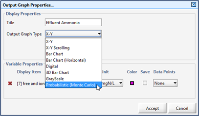
Figure 9‑8 – Output Properties showing Probabilistic Option
Setting up the Input Controller and Distribution Properties
1. Specify the model parameter to serve as the independent variable (see Creating A Control From An Independent Variable in CHAPTER 6).
2. Enter the minimum and maximum value for the independent variable and set it as the Analyze – Monte Carlo controller type (see Input Controls Properties in CHAPTER 6).
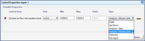
Figure 9‑9 – Set Input Control to Monte Carlo Type
When Analyze – Monte Carlois selected from the drop-down menu, a button will appear beside the Type column. Clicking on this button opens the Distribution Properties dialog for the Monte Carlo analysis.
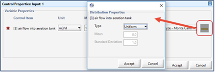
Figure 9‑10 – Accessing Distribution Properties
The probability distribution may be defined as uniform, normal, or log normal. The particular normal or log normal distribution required is specified using its mean and standard deviation.
3. Select the Monte Carlo analysis from the drop-down list accessed through the Analyze button on the Main Toolbar (see Figure 9‑5) or the Analyze menu item in the Tools Menu.
The status bar at the bottom of the main window will indicate that you are in Analyze Mode.
4. Select the desired Stop Time (if applicable) and start the simulation.
During each run, by default GPS-X selects a new set of random variables from the designated distributions. If a repeatable set of random variables is required, change the “Monte Carlo seed” value in the View > Preferences > Input/Output menu to a positive value. Setting the seed value to -1 will force GPS-X to select a new set every run.