CHAPTER 8

Building and Running a Model

Dynamic Modelling & Simulation

Dynamic modelling in wastewater treatment starts with a formal description of the relationships between variables in unit processes; that is, development of models. This task of synthesis has been one of the primary bottlenecks in the application of models to wastewater treatment. Over the years, an extensive effort has gone into formalizing models of different unit processes in wastewater treatment. These models have matured to the point where they are valuable tools for the practitioner.

Models

Models are computer representations of real systems. The real systems of interest here are the unit processes in a wastewater treatment plant, such as the aeration basin or the sedimentation tank in an activated sludge treatment system. Models in GPS-X can be classified as either mechanistic or empirical. The difference between empirical and mechanistic models is more a continuum than a rigid classification as mechanistic models often have some empirical component.

Mechanistic models (Figure 8‑1) are based on first principles, that is, laws of physics, chemistry, and biology. Actual data are used to modify parameters in these models. For example, the law of conservation of mass is the essential building block on which dynamic equations are based in GPS-X. Data collected in the real system are used to adjust physical dimensions, rate constants and other parameters in the equations. This is a "bottom-up" approach to modelling in which the model is provided a firm foundation by natural laws. These laws help us to understand more thoroughly the behavior observed in the real system and the model. Many of the models in GPS-X are mechanistic.

Empirical models rely solely on data. In this approach, the model structure is determined by selecting from a set of general mathematical expressions such as those shown in the center of Figure 8‑2. There is no guarantee that the selected model will be ‘correct’. Essentially, the data "speak for themselves" and ultimately dictate the form of equations - selected among a set of candidate equations on the basis of goodness-of-fit - to be used in the model.

This "top-down" approach to modelling is weaker than the mechanistic approach as the model structure is simpler and the meaning less clear. A different set of data can often result in a different model structure, and we are not always certain how to interpret the meaning of parameters in the model. Nevertheless, empirical models are useful as long as their use is limited to the data ranges over which they were fitted, and in many cases, are the only choice when we have limited knowledge about the real system being modeled. For example, empirical models often give good predictions and can ultimately lead to the discovery of more general mechanistic expressions. GPS-X includes several kinds of empirical models. In these models, actual data determine which model to select and the values of parameters in the selected model.

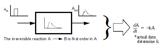
Figure 8‑1 – Mechanistic Models are Based on First Principles

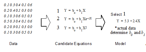
Figure 8‑2 – Empirical Models Fit the Data to a Certain Model Form

State and Composite Variables

The system of differential equations, which GPS-X automatically generates in the model building process, constitutes a precise mathematical representation that describes the relationship between model variables. Some of these variables, referred to as State Variables, are important because they define the “state” of the system[8]. In the absence of any external excitation, the state variables determine how the system behaviour evolves over time. Secondary or composite variables are calculated from state variables and other constants, so they always depend on how the state variables change. The difference between these two variable types is demonstrated in Figure 8‑3.

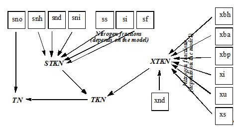
Figure 8‑3 – Nitrogen State (Boxed Variables) and Composite (Bolded Text) Variables

The essential behaviour of a model is closely linked to the response of the model’s state variables. This is a key to conducting effective sensitivity analyses. You can examine the behaviour of composite variables, and this is convenient as composites are often the kind of variable typically measured in a plant, for example, mixed-liquor suspended solids is a variable composed of several particulate state variables. As shown in Figure 8‑3, Total Kjeldahl Nitrogen (TKN) is a composite variable calculated as the sum of soluble and particulate nitrogen state variables plus the nitrogen fractions of some organic state variables. State variables are the basis on which models are organized in the GPS-X libraries.

State Variables and GPS-X Model Libraries

Models are approximations of a real system. State variables are the essence of a model, but it was not described how these are selected. Given assumptions about the proper state variables, another problem is identifying the reactions that these variables undergo. This includes specific expressions for the reaction rate (kinetics) of each variable and the mass ratios (stoichiometry) between variables.

In many cases there are obvious choices for state variables, such as substrate and biomass concentrations in the activated sludge process, but in general this requires care in selection. Simplifying assumptions must be made and these are reflected in the specific choice of state variables. Modelers always try to find a balance between model complexity and prediction capability as shown in Figure 8‑4. Increasing the complexity of a model by adding new reaction terms, etc., may increase its ability to make more accurate predictions but it carries extra overhead including more difficulty in comprehending the model structure, additional data requirements and reduced calculation speed. Removing or simplifying reaction terms minimizes these problems but may result in less accurate predictions. No single model can explain all real system behavior under all circumstances, so it is important to have flexibility in selecting the model to be used for a particular purpose.

GPS-X gives you the necessary flexibility in model selection by providing a number of libraries containing many state-of-the-art models. The model libraries available with GPS-X are shown in Table 8‑1.

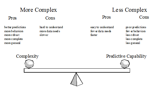
Figure 8‑4 – Balancing Multiple Objects is Important in Developing a Good Model

Table 8‑1 - Model Libraries Available in GPS-X

Library Name	Number of State Variables
Comprehensive (Mantis2)	52
Sulfur and Selenium (Mantis2S)	72
Greenhouse Gas/Carbon Footprint (Mantis3)	56
Process Water (Procwater)	68
Petrochemical (Mantisiw)	52
Carbon – Nitrogen (CN)	16
CN Industrial Pollutant (CNIP)	46
Carbon – Nitrogen – Phosphorus (CNP)	27
CNP Industrial Pollutant (CNPIP)	57

You have a choice with regard to the basic state variables you can model. You can get more information on each of these libraries in the Technical Reference.

A Common Basis for Models

Now that you are familiar with the general nature of unit process models available in GPS-X, you may question how the GPS-X system manages the integration of different kinds of models. In GPS-X, state variables are the elements common to every model in a library. As these are the essential variables, they provide a convenient basis for combining different unit process models. All models in a library include expressions for each of the state variables. The values for these variables at entrance and exit points are particularly important because these are the points at which flows to and from other processes originate or terminate. To build a multi-unit-process model, it is necessary to track these values between unit processes.

The key task of tracking state variables between unit processes is handled transparently by GPS-X.  GPS-X manages this in a rigorous way.  You can display the values of these and other composite variables at every point in your plant layout, but you can ignore the procedures for mapping the state variables among the models. This is another example of how GPS-X insulates you from unnecessary detail, increasing the power of the models you are able to build and allowing you to concentrate on understanding your model and your system rather than code implementation.

Material Balance Expression

One of the key tools of practitioners in engineering is the material balance. Construction of dynamic models is a straightforward application of this fundamental principle. When GPS-X builds a model of a layout, it does so by first establishing the material balance for each state variable in the unit process. As discussed above, this involves tracking the state variables in each unit process in the layout. This is the essential task of the GPS-X translator, which converts the graphical layout into code as described in the Overview of The Model Building Process section and shown in Figure 8‑10.

The material balance expression for a constant volume can be stated as:

The net rate of change in a component within a control volume (an object in GPS-X) is equal to the rate at which the component enters the volume, minus the rate at which it leaves the volume plus or minus the rate at which the component is generated or used within the volume.

This is shown graphically in Figure 8‑5. For each object in GPS-X a material balance dictates the changes which occur in the key components, that is, the state variables.[9] All other dynamic characteristics of the system depend on how these state variables change. There may be several hundred equations constructed by GPS-X if the layout is large. Both steady state and dynamic (time varying) situations can be analyzed using the same fundamental relation and the equations produced by GPS-X.

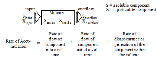
Figure 8‑5 – Material Balance Expression for Two Components (State Variables) and X

Steady-State and Dynamic Simulation

From the material presented in the previous sections, you should now have a general understanding of the nature of the models in GPS-X and the way they are constructed. In the last section, it was stated that the equations can be used for analysis of both steady-state and dynamic, or time-varying situations. The important differences between these types of analyses are examined in this section.

Steady-State Analysis

Steady-state analysis assumes that none of the state variables change over time. To get a qualitative feel for the meaning of steady-state, assume a situation where a plant has been operating under the same external excitations for an extended period of time. The plant has been receiving the same influent, with the same composition and has been operated in the same mode for several months. The situation is shown in Figure 8‑6. In this scenario, the influent flow and operational mode are potential sources of external excitations, but for the moment assume that they do not change over time. As none of these changes, after some time, the plant settles into a steady-state. Because no external excitation is disturbing the plant, variables measured in the plant, such as DO and MLSS, do not change during the period, that is, the variables are not dependent on time. Whenever you interpret the results of a steady-state analysis, remember that the results are valid only for a plant operating at steady-state as described here.

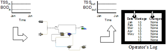
Figure 8‑6 – A Treatment Plant Operating at Steady-State

Finding state variable values at steady-state involves an iterative procedure for solving a system of simultaneous equations. Normally, this procedure converges (finds the solutions) but sometimes it does not. In the latter case, the state variable values contain a (possibly high) degree of error. Ensuring that these errors are kept to a minimum is an important consideration because if a solution cannot be found there may be a problem with the structure of the model or the parameter values being used. Whenever you conduct a steady-state analysis, make sure that the solution procedure converges to a reasonable state. The steady-state solver included with GPS-X is a robust procedure that was specifically designed for the types of models used in wastewater treatment facilities. See the Steady State Simulationsection in this chapter for more information.

Conducting a steady-state analysis of a model is a convenient way to get a feeling for model variable relationships. Values calculated by the steady-state solution procedure depend on the values of all model inputs and parameters. For example, the steady-state value for effluent ammonia depends on the value for the wastage rate because this affects the growth of ammonia-removing bacteria. One quick way to see the relationship between wastage rate and effluent ammonia concentration is to conduct a steady-state sensitivity analysis. To do this, simply change the value of the wastage rate, run the GPS-X steady-state solver and observe the calculated value for effluent ammonia. Do this for several different wastage rates to see the effect over a range of wastage rates. This can be done manually or automatically if you have purchased the Analyzer option in GPS-X.

Dynamic Analysis

The assumption of steady-state is convenient, but most plants do not operate in steady-state. For most realistic situations, it is important to conduct dynamic sensitivity analyses to observe the time-dependence of variables. This situation is shown in Figure 8‑7. In contrast to Figure 8‑6, this plant is in a continuous state of change. The influent composition varies and operational changes, process upsets and equipment failures disturb the steady operation of the plant.

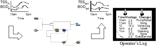
Figure 8‑7 – A Treatment Plant Operating under Dynamic Conditions

Dynamic analysis gives a more complete picture and can serve to validate or reinforce the results of steady-state analysis. Most plants do not have a constant, unchanging influent, and are subject to frequent disturbances (excitations) that result in wide fluctuation in the values of measured variables. For wastewater treatment facilities, dynamic operation is the norm and steady-state operation the exception. This does not mean that results from steady-state analysis are invalid because often a dynamic analysis shows that the model variable values lie within a range, which includes the steady-state value; however, it is always a good idea to supplement a steady-state analysis with a dynamic one in cases where you suspect that the plant is significantly influenced by dynamic disturbances.

Integration Error and Instability

The benefits of dynamic simulation are significant; however, the solution of the dynamic equations is more complex and, if done correctly, can introduce errors in the results. The two major considerations in the solution of dynamic model equations are numerical instability, and the error between calculated and actual values (referred to as convergence). GPS-X is designed to minimize these types of problems. For the great majority of simulations you perform, the default conditions imposed by GPS-X will ensure adequate accuracy of the solution to the model equations. GPS-X includes robust procedures for this purpose and makes it easy for you to apply them in conducting simulations.

Dynamic analysis requires numerical integration of the model equations, that is, the estimation of derivatives by finite difference approximations for each of the model’s state variables. When using these procedures, there is always a small error, referred to as the integration error, between the calculated value and the real value, which would be obtained from an exact solution of the equations. You can control this error by setting integration method parameters or by selecting a different integration method. There are several methods available in GPS-X and you can easily change from one method to another. In most cases, it is possible to keep this error below a reasonable, arbitrarily selected limit.

The second consideration that sometimes arises in numerical simulation is instability. Under some circumstances it is possible for integration procedures to become unstable. The effects of this may be minor, such as small, rapid changes in the value of a variable, or they can be dramatic, resulting in the invalidation of a simulation run. These problems typically occur when using one of the less robust integration routines, especially if the integration step size is made too large. This may be done for convenience or to save time as the large step size requires fewer calculations and therefore, results in faster execution times.

A simple way to determine if errors or instability are a problem is to run the same simulation with more than one of the available integration methods. If you find significant differences in the results of these runs, then one of the methods is producing incorrect results. Try making adjustments to the integration parameters and re-run the simulations until you get agreement between the results calculated by different integration procedures. Consult the GPS-X Technical Reference for more information on this topic.

Initial Conditions

Finding solutions to the dynamic equations, which comprise the models you prepare with GPS-X, is referred to as an initial value problem. In general, the behaviour of a dynamic model depends on:

1. The model equations,

2. The values of parameters and inputs to the model equations,

3. Inputs to the model (forcing functions), and

4. The initial values of the model state variables.

Without assigning initial values to the variables, it is not possible to find a unique solution to the set of differential equations that comprise the model. In previous material we have described how GPS-X constructs the model equations and the ways for you to enter model parameter values. The remaining task is to select the initial conditions. As the behavior you observe is dependent on these values, it is useful to take time to consider how initial values can be determined and how the results you obtain should be interpreted.

In all the simulations you perform with GPS-X, it will be necessary to specify the initial conditions. There are two ways to do this:

1. Enter the values directly, and

2. Calculate the steady-state values at time=0 and use these as the initial values.

The procedures for setting the values directly have already been covered in the Process Data Menu sections. As initial values are a kind of model attribute, their values can be set from the object process data menu. The hierarchical menu obtained by selecting this item is shown in Figure 8‑8.

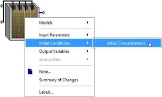
Figure 8‑8 – Initial Conditions Menu Item

Remember that the initial values determine the unique solution obtained for the set of defining (differential) equations. If these values are set directly, then you must take care in making a proper interpretation of the meaning of the simulation results obtained. A safe way to set the initial values, one with a simple interpretation, is to use the steady-state solver to calculate the steady-state values and then use these as the initial values.

As shown in Figure 8‑9 there are actually two cases to consider. In case 1, shown on the left-hand side of Figure 8‑9, the process has been at a steady-state prior to the start of the simulation (t=0). After starting, the changes made to model inputs or parameters cause some dynamic behavior to occur. This is the case mentioned above, where the steady-state solver has been used first to calculate the steady-state. After doing so, the state variables are given these steady-state values at the starting time (t=0). The state variables at any time after the start are influenced by changes to model inputs or parameters resulting in the dynamic behavior you observe.

In the second case shown on the right-hand side of Figure 8‑9, the behavior of the state variables is dynamic before and after the point where time=0. Consider two additional scenarios of Case 2 that may be simulated; one in which there is no knowledge of the dynamics before time=0, and one in which there is knowledge of the dynamics before time=0.

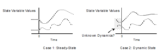
Figure 8‑9 – Two Possible Simulation Cases and their Relationship to Initial Values

If there is no knowledge of the dynamic behavior before time=0 and the initial values are entered directly, perhaps from actual measurements or based on engineering judgment, then it is not always clear whether the behavior after time=0 accurately reflects the dynamics in the system being modeled. Relatively small errors in a single state variable initial condition can cause significant errors in the simulation results.

It is also possible to specify a set of initial conditions that violate model validity constraints, for example, entering a negative value for concentration or an unreasonably large or small value for a state variable. Under these circumstances the integration of model equations may still be stable with a low integration error, but the results are not valid. In general, you should exercise care in the selection of initial conditions for this case.

Given good estimates of the initial conditions, the system of equations will eventually "settle in" to a repeatable pattern. This period can be estimated as it is dependent upon the time constants for the processes being modelled. In wastewater treatment processes, important time constants are the hydraulic detention times of the unit process and the sludge age, or solids retention time (interpreted as the mean age of the solid matter) of a system of unit processes, for example, the activated sludge process. Generally, a value of 2 to 3 times the hydraulic or solids retention time should be used as a minimum period.

If there is knowledge of the dynamics before time=0 then it is possible to determine exactly the derivatives and, therefore, the behavior of the system. This would be the case if you restored the initial conditions from a previous run or when there is a repeating pattern of model inputs or parameter changes, such as a repeating diurnal variation in influent flow rate and composition. For the latter case, you may at first only have estimates of the initial conditions, but you can determine the exact initial conditions by re-running the simulation with the same inputs until you get identical results for consecutive runs. GPS-X includes this capability and will perform the necessary re-runs automatically.

You have many options in setting-up and running simulations. In some cases, it is not necessary to run dynamic simulations because you can get the information needed by completing a steady-state analysis. In other cases, extensive dynamic analyses are necessary. For example, a simple treatment plant design might require only steady-state values, whereas an on-line application may necessitate closer attention to process dynamics.  Take some time to think about the results obtained to ensure that the simulation results are understood correctly. GPS-X helps you to get the simulations right - interpreting correctly is up to you.

Overview of The Model Building Process

The build procedure is shown in Figure 8‑10. In GPS-X descriptive models are supplied in libraries. When you place objects on the drawing board and specify their Model types, GPS-X knows which models to retrieve from the library. When you specify the connections between objects, GPS-X then knows how to couple these models to generate a dynamic model of the entire layout. As default data are defined for all critical model parameters, it is possible to translate the layout into a high-level computer language and generate an executable program.

In GPS-X, the model build process is transparent; once you have prepared the layout on the drawing board, creating an executable model is done when switching over to Simulation Mode. GPS-X achieves this using a specialized translator, which converts the graphic images you place on the drawing board into dynamic model equations. Once the executable code is generated, you can conduct simulations of the model.

Figure 8‑10 – The Model "Build" Process in GPS-X

As shown in Figure 8‑10, GPS-X simplifies the construction of models by automating many tasks with special routines. The first step involves the GPS-X translator, which is a special pre-processor program that converts the layout you prepare to a high-level description of a dynamic model. The GPS-X translator writes the material balance equations for each unit process based on the models and connectivity you specified. Many levels of detail, which concern the mechanics of constructing the code rather than process understanding, are hidden through the use of an extensive macro language. This allows you to concentrate your efforts on understanding the model itself rather than the modelling and simulation tools.

The remaining steps in the build process do not require user interaction. The GPS-X translator writes a high-level description of the model in the Advanced Continuous Simulation Language (ACSL^TM). ACSL is a third-party program that is used as the simulator module in GPS-X. ACSL handles the details of numerical simulation, including the ordering of equations, integration, and many other details. In the next step, ACSL code is converted directly to a FORTRAN program, then to object code, and finally to an executable module. The entire build process can take less than a minute to complete, even for moderate-sized models. When you run a model in GPS-X, you are running the executable module shown in Figure 8‑10.

Building a Model

When switching from Modelling Mode to Simulation Mode (see Modelling/Simulation Mode section in CHAPTER 1), if necessary, the numerical model will be built.

If the model for this layout has previously been built, but the layout has been modified, you will be prompted to rebuild the layout or simulate with the older version of the model (in most cases, you will want to rebuild the model).

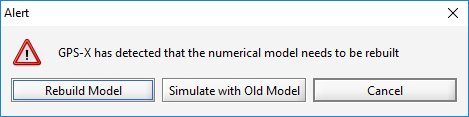
Figure 8‑11 – Rebuild Model Option

When the model is being built, you will see the “Building Model” window, as shown in Figure 8‑12.  The status of the building process will be updated as it moves through the different steps and any errors that occur will be displayed in this window.

Building the numerical model may take from 5 seconds up to a couple of minutes, depending on the speed of your computer and the complexity of your model. When the model building is complete, the “Building Model” window will automatically close, and the model will be ready for simulation.

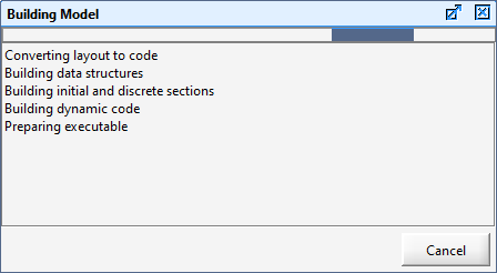
Figure 8‑12 – Building Model Dialog

Building Options

NOTE: This section is for advanced users. Unless you are interested in the details of the model building process, you can skip forward to the section on Starting Simulations.

The build process, while fully automated, can also be carried out manually from the Tools > Buildmenu while in Modelling Mode for those situations where you may want to test whether a model will build without an error, but you are not ready to move on to running simulations yet.

The process of building involves two major steps:

1. Translating the drawing board layout to ASCL source code.

2. Compiling and linking the source code to produce a FORTRAN executable program.

All messages related to the build process will be displayed in the Building Model window (Figure 8‑12).  This includes the GPS-X and ACSL translator messages, compiler messages and linker messages.

If the build process is successful, the window is automatically closed.  Otherwise, it will remain so that you can view what the problem is. Some of these errors can be solved by adjusting the Translation Options.

Translation Options

If you wish to control how the translation step is performed, you can specify building details in the Build tab of the View > Preference menu, as shown below.

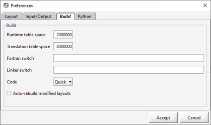
Figure 8‑13 – Preferences Dialog (Build Tab)

The Code item has several options for the code generation step.  The Quick option creates code optimized for speed whereas the Big and Big+options are used for large treatment process models. These options are described in greater detail below.  If you make changes to the code generation options, you must subsequently select the Tools > Build menu item to prepare the executable program.

QUICK Option

Many GPS-X models contain recycle streams between processes. To find an accurate solution to the model equations in these cases, the numerical solution routines must iterate at every time step to resolve the effects of changes occurring in upstream units or downstream units, which in turn, may affect upstream units via recycle streams.

At any point receiving a recycle, the (numerically integrated) components of the recycle stream cannot be known accurately until effects are propagated through the plant to the source of the recycle. At some point, a balance is struck, but finding this balance requires an iterative solution. The Quick option ignores these effects and the computational overhead associated with them. Using the Quick option effectively reduces the execution times.

The difference in model predictions made using the Quick option and the exact solution are usually not significant. This is because integration time steps are much smaller than the time constants of processes in a typical wastewater treatment plant and the changes, which occur between time steps, are small. For most purposes, the Quick option is the best choice. The Quick option is assumed if you select the Build menu option.

BIG Option

When building a large plant model containing many unit processes (for example more than 10 settlers) it is possible to exceed the limits which the simulator module places on the number of discretely executed code sections.

When this occurs, the translation to source code will fail and an error message (‘too many discretes, build BIG’) will be displayed in the Building Model window.  In most circumstances, GPS-X will auto-detect when a build fails with a “too many discretes error”, and automatically rebuilds the layout with the BIG option.

When the BIG option is used, all controllers in the layout use the same discrete sampling interval, rather than individual sampling intervals specified in each object.  This controller sampling time is specified in the Layout > General Data > System > Inputs Parameters > Dynamic Solver Settings menu.

BIG+ Option

This option is similar to the BIG option. Instead of defining a single sampling interval for all controllers, scalar PID controllers (only) are disabled.

Starting Simulations

GPS-X allows you to conduct simulations interactively rather than (or in addition to) batch model simulations. Interactive simulation is simple – you Start the model and then change the pre-defined controls to observe the response of model variables set up in output displays. There are some useful set-up commands, which you may want to issue before beginning and you can interrupt the simulation at any time, query the simulator for specific variable values, modify the displays or controls and then continue with the simulation. GPS-X is designed to make this interaction easy in order to get the maximum amount of information from a simulation run.

Steady State Simulation

To start a steady-state simulation:

	1. Make sure you are in Simulation Mode
	2. Select Steady State on the Simulation Toolbar.
	3. Enter a value of 0.0 for the Stop Time.
	4. Click on the Start button.

The simulator will then run the steady state solver and pause when it has reached convergence. The percentage convergence is shown dynamically on the progress bar on the Simulation Toolbar.

If you have the Command Window displayed, the status of the steady state calculations is displayed dynamically.  This information consists of the following: the iteration number, the number of loops without improvement, the current value of the sum of derivatives and the lowest value of the sum of derivatives are shown. Messages indicating whether convergence was or was not achieved are also displayed in this window.

In some cases, the steady state solver does not converge; however, simply re‑running the solver may result in convergence. This is done automatically in GPS-X if the number of retries is set to a value greater than zero (0).

To set the number of steady state solver retries:

1. Switch to Modelling Mode

2. Select the Layout > General Data > System > Input Parameters > Steady‑State Solver Settings menu item. The steady-state solver parameters dialog is displayed as shown in Figure 8‑14.

3. Change the value of Number of Retries on Iteration. A value of 5 or less is best.

4. ‘Accept’ to close the dialog.

5. Switch to Simulation Mode. You will be prompted about rebuilding – select “Rebuild Model”. This will create a new model with 5 (or fewer if convergence is achieved) steady-state retries as default.

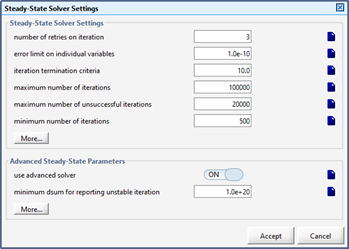
Figure 8‑14 – Steady-State Solver Settings Dialog

An alternative procedure would be to set the number of retries in a scenario rather than changing the layout. This method does not require re-compilation (see Using Scenarios section of this chapter for more details).

GPS-X will re-initialize the steady-state solver and attempt to find a solution to the equations. The number of retries should be kept small as it is unlikely that the system will converge if the procedure has failed after 5 retries. Under these circumstances, it still may be possible to achieve convergence by modifying other solver parameters shown in Figure 8‑14. As a last resort, it may be necessary to modify either the model structure or model parameters to achieve convergence.

Refer to the Technical Reference for more information on the steady-state solver and strategies for modifying steady-state solver parameters.

If the stop time is set to 0.0, the steady-state solver stops after calculating the steady-state values. If the stop time is set to a value greater than zero (0), the simulator sets the initial conditions equal to the steady-state values and starts a dynamic simulation.

Dynamic Simulation

When performing a dynamic simulation, the simulator will always stop when it gets to the indicated Stop Time value; therefore, before starting a simulation, make sure the current value of Stop Time is greater than zero (0).

To start a dynamic simulation:

	1. Make sure you are in Simulation Mode
	2. Select Steady State on the Simulation Toolbar (optional).
	3. Enter a value greater than zero for the Stop Time.
	4. Click on the Start button.

As discussed in the Initial Conditions section in CHAPTER 4, the initial conditions can be set either by entering the values directly or by calculating the steady-state values and using these as the initial conditions.

When steady-state is selected, the steady-state solver starts and the state variables values calculated by the solver, are used as the initial conditions.

If steady-state is not selected, the simulator takes the pre-set initial conditions[10] and immediately begins a dynamic simulation run.

In the former case, there will be a delay before the results begin appearing on output displays as the steady-state solver runs.

The simulator will continue until it reaches the stopping time.

In the Initial Conditions section, problems associated with using estimates for the initial conditions were addressed. The best situation is one in which a repeating pattern of model inputs can be assumed. In these cases, it may be necessary to run the same simulation several times before the system reaches a dynamic, or periodic, steady-state. These additional simulations are performed automatically in GPS-X if the number of re-runs is set to a value greater than zero (0).

To set the number of dynamic simulation re-runs:

1. Switch to Modelling Mode

2. Select the Layout > General Data > System > Input Parameters > Simulation Run Settings menu item. The dialog window is displayed as shown in Figure 8‑15.

3. Change the value of Number of Reruns.

4. ‘Accept’ to close the dialog

5. Switch to Simulation Mode.  You will be prompted about rebuilding.

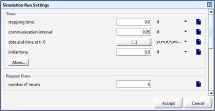
Figure 8‑15 – Simulation Run Settings Dialog (Repeat Runs)

In most cases, Steps 2-5 are made in a scenario rather than the layout (see Using Scenarios section of this chapter). The number of re-runs you select will depend on estimates of the time needed for the system to come to a periodic steady-state. This estimate can be based on important time constants in your system, for example, the detention times of unit processes or solids retention times in combinations of unit processes such as the activated sludge process.

Pausing/Resuming the Simulation

	Whenever the simulator is running, you can pause the simulation by pressing the Pause button on the Simulation Toolbar. Once the simulator paused, you can adjust the interactive input controls, issue commands, alter the integration attributes, etc. After making any changes, you can continue the simulation.
	To resume a simulation when the simulator has been paused, press the Resume button. The simulation will continue from the point at which it was previously interrupted. You can pause and resume as many times as you want during a simulation session.

Output Variable Form

Normally the variables of interest are displayed in graphs which are defined by the user (e.g. bar graphs, XY graphs, etc.). However, at times it is convenient to view the values of variables that were not included in these displays.

One useful feature for quickly checking the values of certain variables is the ability to browse the output variable forms of the various unit processes in your layout.

1. Make sure you are in Simulation Mode

2. Right-click on the object of interest on the drawing board. The object’s process data pop-up menu will be displayed.

3. Select the ‘Output Variables’ item and browse the submenu system to find the category of interest.  Select the item and the Output Variable Form will be displayed.  The current values of the variables are displayed on the form.

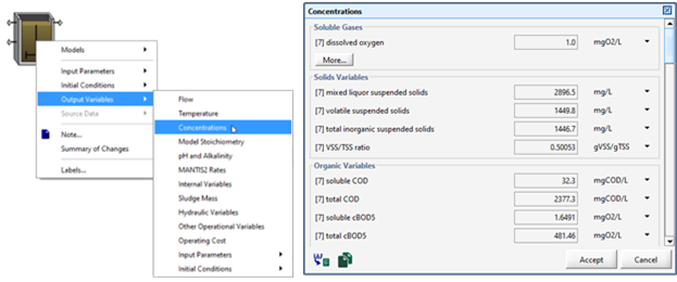
Figure 8‑16 – Accessing Output Variable Forms

Simulation Control

On the Simulation Toolbar there is a button to access various settings regarding the simulation and some different low-level commands that can be sent to the model.

Integration Control

This item allows you access to the window that contains relevant information for the internal numerical solver.  Note that these values can only be altered in a scenario (see Using Scenarios) or in Modelling Mode by accessing the same parameters through Layout > General Data > System > Input Parameters > Dynamic Solver Settings.

Properties

This item allows you access to the settings (ie. min/max/delta) for the Stop, Communication andDelay data entry fields.

Commands (Advanced Users)

When in Simulation Mode, and whenever the simulator is in the idle state, it is possible to query the simulator directly by issuing ACSL runtime commands. These commands can be used to exercise the model, that is, to run a simulation, look at the results, and change model constants.

Most of the essential commands and coordination with the simulator are handled by the GPS-X interface; however, you have the ability to issue ACSL commands directly.

A full description of the ACSL commands is given in the ACSL Reference Manual (contact Hydromantis/Hatch for details).

NOTE: Commands issued to the simulator are executed in the order given and data values that are set remain the same until they are changed by a subsequent command or the model is unloaded. These commands can conflict with GPS-X instructions to the simulator. For example, if you set the value of a model parameter in a GPS-X process data entry form and then later use the runtime command “set” to set the value of the same variable, the latter action will override the former and the value displayed in the GPS-X data entry form will be incorrect.

Eight commonly used commands or procedures[11] are pre-defined and provided in the Simulation Control > Commandsdrop down menu on the Simulation Toolbar, as shown in Figure 8‑17.

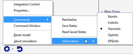
Figure 8‑17 – Simulation Control (Commands Submenu)

Five of these procedures are accessed from the Information sub-menu. They concern information messages that are sent to the Command Window.

These procedures are:

1. Noinfo – suppresses the display of GPS-X system and simulator module messages.

2. Fullinfo – displays all messages.

3. Warninfo – suppresses the simulator module messages, but displays GPS-X system messages.

4. Optinfo – sets up the Command Window for display of optimization information in optimize mode (see CHAPTER 10).

5. DPEinfo – sets up the Command Window for display of dynamic parameter estimation information (see CHAPTER 10).

Information on the messages that are displayed can be found in the Technical Reference.

The remaining pre-defined commands in the Simulation Control > Commands menu are provided for saving and restoring or reinitializing the model state variables.

1. Reinitialize procedure writes the current values of the state variables into their corresponding initial conditions. This is useful for establishing a starting point for a subsequent simulation run. This procedure stores these initial conditions in memory only. It does not overwrite the values that a user sees in the initialization forms, so if the model is unloaded and reloaded, the form values will be used as the initial conditions. The reinitialized values will be lost when the model is unloaded.

2. Save States procedure saves all model data, including state variable initial conditions to a data file.  This file has a pre-determined name (ie. ACSLSV.gps) and is located in the same directory as the layout file, so only one set of model data can be saved at a time using this feature.

3. Read Saved States procedure restores the file output created using the Save States command. This is another useful way to save the data at a point in the simulation so that you can later start a simulation at the same point

Any messages or other output from the simulator module will be displayed in the Command Window.

Command Window

The Command Window is an auxiliary output area used to report details of the system and model status. These include messages that might be generated during run-time.

In addition, the Command Window is the primary text-based output interface to the simulator module.

You can issue commands to the simulator (as described in the section above) or any other valid ACSL command (see Technical Reference for more details) and see the responses in the Command Window.

To display the Command Window:

1. Switch to Simulation Mode (if not already there).

2. Click on the Simulation Control button on the Simulation Toolbar, and select Command Window. The command window will be displayed as a tab in the Output section of the main window.

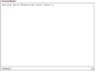
Figure 8‑18 – Command Window Tab

The ACSL commands can be typed in the field at the bottom of the window (see Figure 8‑18) and sent by either pressing ‘Enter’ or clicking the ‘Command’ button.

Using Scenarios

When organizing simulation runs it is useful to start with a base set of data, and then create one or more separate cases, which are modifications to the base data set. These cases are referred to as scenarios in GPS-X.

You can create any number of scenarios and in each scenario, you can specify the changes to the model parameter(s) which define that scenario.  Those changes are saved so that they can be restored at any point in the future.

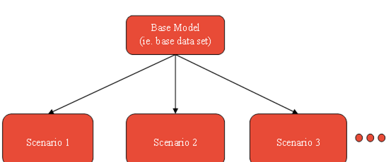
Figure 8‑19 Scenarios Derived from a Base Data Set

A couple of rules that apply to scenarios:

· Scenarios can only be selected at the start of a simulation. This means that if you pause a simulation and then change the scenario, the simulation will no longer be able to be resumed.  It will have to start from the beginning again.

· Changes to model parameters which would require rebuilding the model, cannot be placed in a scenario. For example, it is not possible within a scenario to change the number of reactors in a plug-flow tank, the number of layers in a sedimentation tank, or delete unit process objects. You can, however, set the volume of a tank to zero to make it appear that the tank is not present.

The Scenario menu can be accessed through the Scenario item on the Simulation Toolbar.

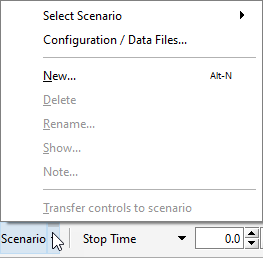
Figure 8‑20 – Scenario Menu

Creating a New Scenario

To create a scenario:

1. Make sure you are in Simulation Mode

2. Click on the Scenario item on the Simulation Toolbar.

3. Select New. A dialog window will be displayed that allows you to select either the default scenario or another existing scenario to derive the new scenario from.  If you select the default scenario, then you are starting from the base case. If you select another scenario, then all the variable changes in that scenario will be copied to the new scenario as a starting point for the new scenario.

4. Type in a scenario name. Any contiguous alphanumeric name can be used.

5. Click the Accept button to create the scenario.  This will also make it the active scenario.

Now you can go to the drawing board and access any of the object’s process data menus to make the desired changes to the parameters. The title bar of the data entry form contains the message – SIMULATION IS LOADED – to indicate that you are in a simulation mode, and that any changes made will be added to the scenario.

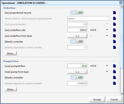
Figure 8‑21 – Scenario Data Entry Form (Changes shown in Green)

Note that all parameter values that are changed as part of a scenario are shown in bold green text in data entry forms, for easy identification.

Selecting the Active Scenario

The currently active scenario can be selected by accessing the scenario menu on the Simulation Toolbar and choosing the desired scenario from the “Select Scenario” submenu.

The active scenario is displayed on the status bar below the Simulation Toolbar.

Figure 8‑22 – Display of Active Scenario

Scenario Configuration

From this dialog window, you can control various aspects of the scenarios.  There are four main features:

1. Add/remove/view data files.  See the Adding Input Files to a Layout section in CHAPTER 6 for more information.

2. Comparing two or more scenarios to see the differences in tabular format.

3. Deleting scenarios.

4. Reordering the list of scenarios.

Viewing Scenario Variables

On the Simulation Toolbar, you can use the Scenario > Show.. dialog window to view the list of variables that have been changed (from the base scenario settings) in the currently active scenario. The base scenario variable settings appear in a grayed-out box, while the modified values appear in green text and can be directly manipulated from this window.

From this dialog, you can also select one or more of the variables and either:

	1. Delete them from the scenario, or
	2. Transfer Values to layout (ie. base data set).  This means that the selected values from the scenario will be set as the base value and removed from this scenario.  This requires the layout to be automatically rebuilt.

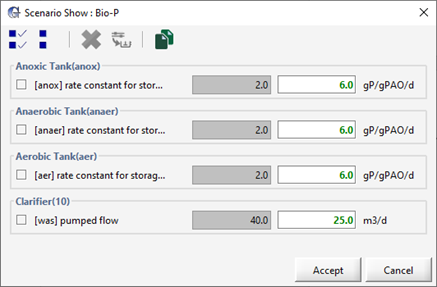
Figure 8‑23 – Example of Scenario Show Dialog

Automating Simulations (Autorun)

The Autorun feature automates a number of common button click events used for running simulations. This automation is done through a text file, <layoutname>.xec that can be created with a text editor and saved with the other layout files. The file contains a sequence of commands which are executed in the order in which they appear in the file.

Following is a list of available commands:

Table 8‑2 - .xec Commands

.xec file commands:
log	DISPLAY LOG WINDOW
scenario <scenario name>	SET SCENARIO NAME
optimize <optimize type>!<objective function>	SET OPTIMIZE TYPE/OBJECTIVE FUNCTION Optimize type is one of: time series or dpe Objective function is one of: absolute difference, relative difference, sum of squares, relative sum of squares or maximum likelihood
Analyzer <analyze type>	SET ANALYZE MODE Analyze type is one of: steady-state, phase dynamic or time dynamic
steady	SET STEADY STATE ON
iconize	START GPS-X IN CLOSED STATE
tstop <tstop> [d/h/m/s]	SET STOP
cint <cint> [d/h/m/s]	SET COMMUNICATION INTERVAL
delay <delay> [s]	SET COMMUNICATION DELAY
command <command>	ENTER ACSL COMMAND
start	START SIMULATION
report	GENERATE REPORT AT END OF RUN
`exit	STOPS ACSL RUN, QUITS GPS-X
help	DISPLAY INFO FILE

The .xec file is executed by default if it exists and GPS-X is started with the –L <layout name> option. This feature can, however, be turned off by using the –x 0 option when starting GPS-X.

Previous Next