CHAPTER 10
Introduction
The Optimize module is used to optimize the values of parameters from your layout. This module is an optional feature. If you have not purchased this module, contact us for pricing information.
The Analysis Tools chapter explained how to use the analyze module to study the behaviour of your models and to identify the important parameters. Once you have identified the important parameters, you can use the optimizer module to optimize the values of these parameters. Optimization involves adjusting certain model parameters to achieve a desired objective function.
The optimizer can be used to fit a model to measured data or to optimize process performance. The procedure of fitting a model to measured data is called “parameter estimation” and involves adjusting selected model parameters to achieve the best possible fit between the model responses and the measured data. Parameter estimation is an important step in preparation of a simulation model because process parameters can vary significantly from plant to plant. A model that has been fitted to actual plant data will be more useful for predicting actual plant behaviour.
Process optimization involves adjusting certain model parameters to maximize or minimize the value of a model variable or a user-defined variable. For example, you may wish to adjust certain model parameters to minimize a plant's operating cost.
The optimizer module was developed specifically to solve parameter estimation and process optimization problems involving dynamic wastewater treatment models. It can be used for both steady-state and dynamic optimization. As will be seen in this chapter, the optimizer is a valuable tool for preparing effective models of wastewater treatment facilities.
Uses of Optimization
There are several areas where optimization can be beneficial. In wastewater treatment, the main areas of application are in model calibration (i.e. parameter estimation), process design, and process optimization.
Parameter estimation is important because once a model has been built it often becomes necessary to fit the model to real data. In fitting simulation results to real data, it is usually found that many stoichiometric parameters can be assumed constant but that physical, operational, and kinetic properties vary significantly from plant to plant. You can use the GPS-X parameter default values as a starting point, but when it is necessary to use the model for purposes of predictive simulation then calibration should be performed. This can be a simple manual or qualitative simulation in which you conduct interactive simulations or a rigorous mathematical one using formal optimization techniques.
Simulator optimization can be used for process design and plant optimization. Consider the problem of finding a plant design that meets certain effluent requirements. Another example is finding the best operating mode to reduce the loss of suspended solids during a plant upset. In both cases, there is a desired output, namely the design that meets the effluent limits and the best operating mode. If you have a model of the system, these objectives are achieved by varying plant design or operational parameters and observing the response of the model outputs.
In GPS-X, you choose the target parameters and the optimized variables of interest, and select an objective function to achieve a desired optimization. There is no limit on the number of response variables. The optimizer adjusts the selected parameters until the objective function is minimized.
Algorithm Used
GPS-X uses the Nelder-Mead simplex method (Press et al., 1986) in the optimizer module. The simplex method is a robust multi-dimensional algorithm that does not rely on gradient information. The algorithm searches through a multidimensional "surface" or space (defined by the objective function) in an organized way to find a path to a minimum value for the objective function. The procedure is sensitive to the choice of the optimization parameters. For more information on the simplex algorithm refer to the Optimizer chapter in the Technical Reference.
Types of Optimization
The optimizer module is equipped to handle three different types of process measurements:
1. Time series measurements,
2. Long term operational data that are averages of the original process measurements, and
3. On-line measurements.
Each type of measurement set leads to a different type of optimization problem. The optimization problem types available in GPS-X are Time Series and DPE.
Time Series
This optimization type is the one normally used for both parameter estimation and process optimization. It is designed to handle both time series and steady-state measurements.
For parameter estimation involving a dynamic model, the data entered into the text file will be the values for each of the response variables that you would like to fit at a series of time values. The response variables are referred to as target variables. In GPS-X, the target variable can also be maximized or minimized.
Steady-State optimization is a time series-type optimization with only one data point for each target variable. The steady-state solver is used, and the simulation has a stop time of 0.0. This type of optimization is useful for calibrating the model to data reported as daily, weekly, or monthly averages. Data of this type is typically obtained from composite samples and do not accurately reflect the time dynamics of the real process. In a steady-state optimization, the average data values are used as the targets and selected model parameters are adjusted to fit these targets.
GPS-X will fit your model to the measured data using the objective function that you select. On the output graphs used to display the predicted values of the model, the measured values provided in the data file will be displayed on the graphs with red diamond markers.
GPS-X will draw a new curve for the predicted values at each optimization iteration, so that you can track the progress of the optimizer. At the end of the optimization run, final predicted responses are displayed so that you can visually assess the fit. An example of this type of graph is shown in Figure 10‑1.
You can use any of the available objective function types when doing a time series optimization. These are listed below:
1. Absolute Difference
2. Relative Difference
3. Sum of Squares
4. Relative Sum of Squares
5. Maximum Likelihood
When doing parameter estimation, the maximum likelihood or sum of squares objective functions should be used. For process design or optimization, the absolute difference objective function is the most suitable. For more detail on the different objective functions see Objective Function Options in the Optimizer chapter of the Technical Reference. The optimization results you obtain can depend strongly on the chosen objective function.
Dynamic Parameter Estimation (DPE)
GPS-X has a sophisticated dynamic parameter estimation feature (DPE) designed for the estimation of time-varying parameters. It can be used with on-line data or off-line time series data. For details on using on-line data, contact Hydromantis/Hatch.
The motivation behind DPE is that parameters in process models are often not constant but vary with time. For example, the oxygen mass transfer coefficient in an aerated tank is often slowly time-varying.
Dynamic parameter estimation is useful for estimating parameters in poorly understood processes. In these cases, the model structure is likely to be incorrect. As a result, the model may only be able to represent the data well over short time intervals. In this case, using DPE will help compensate for the model error and allow acceptable fitting of the measured data.
Another situation in which dynamic parameter estimation is useful is when you are interested in detecting process changes and upsets. If for example a model parameter is found to be relatively constant during normal process operation but is sensitive to process changes, you can track this parameter using the DPE feature and on-line data to help provide an early warning of process changes or upsets.
In GPS-X dynamic parameter estimation is done by applying the time series optimization approach mentioned earlier to a moving time window. Instead of estimating parameters from an entire set of data, GPS-X calculates a set of parameter estimates for each time window using the parameter estimates from the previous time window as a starting guess. This approach can be used on a data file that is continually updated with new blocks of data (online data) or on a static file of time series data. You can use any of the objective functions that are available for time series optimization when doing dynamic parameter estimation.
The length of the time window controls how often the parameters are updated. The shorter the time window, the more often the parameters are updated. When using short time windows, it may be necessary to filter the data to eliminate noise so GPS-X does not fit the noise.
To ensure proper termination of the optimization routine when using the DPE feature, it is suggested that the time window and the communication interval be chosen such that the time window is an integer multiple of the communication interval.
Dynamic Simulation Initial Conditions
When performing an optimization involving a dynamic simulation you can set the initial conditions using the steady-state solver or provide your own initial estimates of the initial conditions. This choice is dictated by the target data and knowledge about the dynamics of the system and its behavior at the start of the simulation.
If the dynamic target data include initial steady-state estimates, perhaps from time-averages, you can use the steady-state solver to establish the initial conditions for the simulation. If you know that the system is not at steady-state at the start of the simulation, you can use the initial data points in the real data set as the initial conditions. Figure 10‑1 shows an optimization of a batch process in which the initial condition represents the initial concentration of soluble substrate in a tank. The target data are shown as discrete points and simulation results for six values of the independent variable are shown as continuous curves. Steady-State initial conditions are not appropriate for this case. Since soluble substrate (a state variable) is utilized in the batch reactor, the steady-state solver would find a solution at zero substrate concentration. If the simulation started at zero initial substrate, the optimizer would not be able to fit the simulation to the target data.
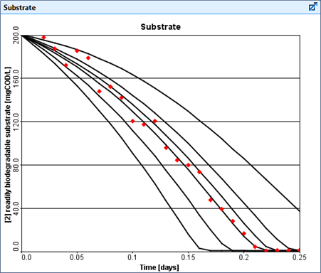
Figure 10‑1 – Example of Dynamic Simulation using Initial Conditions
Selection of the Optimization Variables
Before using the optimizer to adjust parameter values it is usually best to experiment with manual adjustment of the parameters. It is a good idea to familiarize yourself with the models you prepare to understand the important relationships. By conducting interactive simulations, you can observe the effects of the many model parameters on the response variables of interest. With this information, you will be able to make better judgments on appropriate independent and target variables to use in an optimization.
One common optimization problem is selection of improper optimization parameters. In setting up a manual or automatic optimization, be sure to select those parameters that have a significant effect on the specified target variables. For example, effluent ammonia concentrations are highly dependent on, and responsive to, the value of the nitrifier growth rate or reactor aeration parameters, but not so dependent on the value of the carbon-removing organism growth rate. Similarly, recycle sludge concentration is not influenced greatly by the settler model flocculation parameter whereas effluent suspended solids from the settler is influenced by this parameter. As demonstrated by these examples, selection of appropriate optimization variables requires an understanding of the structure of the model.
Including too many parameters in an optimization will result in a difficult optimization problem with a high degree of correlation between the parameters. As a result, the parameter values at the solution will have a high degree of uncertainty associated with them.
When you are satisfied that you know the important relationships and have identified appropriate target (response) variables and optimization variables, it is best to perform some manual optimizations. Set up several interactive simulations with slider controls on the optimization variables and try adjusting these as the simulation proceeds. You can plot actual data along with the target variables (see the Variable Properties section in CHAPTER 7) so that you can compare simulation and actual data. This type of qualitative optimization is helpful in a number of ways. For example, it helps to identify initial guesses and establish practical bounds on the optimization variables.
Steps in an Optimization
Optimization setup must be performed in Modelling Mode.
To run the optimization, you must first fully setup the target variables, optimized parameters, and objective function using the Optimizer Setup Wizard. Once the wizard is completed, the model will automatically re-build to display necessary input and output parameters. The re-build is necessary to embed optimization instructions in the simulation model.
Optimizer Setup Wizard
|
|
The first step in setting up an optimization is to run the Optimizer Setup Wizard in Modelling Mode. Press the Optimize button on the Main Toolbar |
1. The first stage is selecting the desired target variables. Navigate through the variable tree to find and select the desired variable.
The target variables are the variables that you would like to minimize, maximize, or fit to the measured data. The target variables are often the same variables as those you would plot in a normal-mode simulation.
For time series and DPE optimizations you can select other target variables in this way but keep in mind that data requirements and calculation times required for multi-target optimizations can become prohibitive.
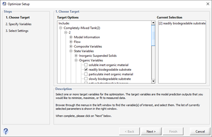
Figure 10‑2 – Optimizer Setup Wizard (Specify Target Variables)
Click “Next” to move on to the next stage.
2. Select the desired optimized variables by ticking the appropriate boxes. The optimization variables will be adjusted by the optimizer as it attempts to minimize the objective function.
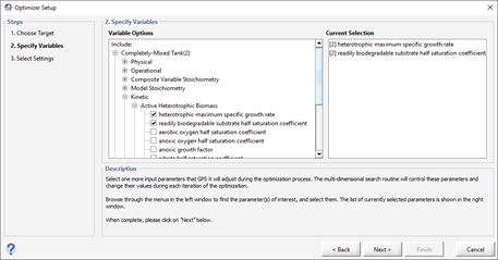
Figure 10‑3 – Optimizer Setup Wizard (Specify Optimize Variables)
Click “Next” to move on to the next stage.
3. Specify the desired target comparison, objective function, and optimization type. The target variables can be minimized, maximized, or fit to an input data. The input data can be imported into GPS-X by selecting Fit to Data under Target Comparison and clicking on the Add Data File button.
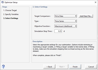
Figure 10‑4 – Optimizer Setup Wizard (Specify Optimizer Settings)
4. Press ‘Finish’. Once you press finish, the model will automatically switch to simulation mode and re-build. Notice that the layout is now in Mode Optimizer- Time Series. A new input tab labeled Optimization Parameters and a new output graph tab labeled Optimization Results will be automatically generated. The Optimization Parameters input tab contains the optimized variables, and the Optimization Results output tab contains the graphs of target variables the user specified.
If you load a layout where the Optimizer Setup Wizard has already been run, the simulation will be in ‘normal’ mode. To turn on the optimizer, press the Optimize button on the Main Toolbar.
The optimization type and objective function can also be changed in Simulation Mode instead of re-running the wizard. For details on how to do that, see the description of the Optimize menu in CHAPTER 1.
Running the Optimizer
To conduct an optimization, you must be in Simulation Mode, and you must turn on the optimizer (if it is not automatically turned on after going through the Optimizer Setup Wizard described above).
To run an optimization, complete the following steps:
|
|
1. Be sure you are in Simulation Mode. |
|
|
2. Click on the Optimize button to switch to Optimize Mode. Alternatively, you can right-click on the inverted triangle beside the optimize icon, and then select Optimize Mode. If you have not selected the Type and the Objective Function, do this now. A message indicating you are in Optimize Mode will be displayed in the status bar. |
|
|
3. Set the Stop Time and the Communication Interval to the desired values. |
|
|
4. Click on the Start button on the Simulation Toolbar. |
As the optimization proceeds, on the output graph several different simulation curves will be overlaid and these curves should begin to converge to the real target data.
The number of curves shown on the graph can be set by going to View > Preferences and on the “Input/Output” tab setting the Number of runs displayed (analyze/optimize)parameter.
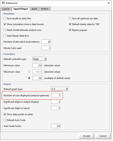
Figure 10‑5 – Preferences (Number of Runs Displayed)
You can watch the input controllers to get a feel for the way the optimizer makes changes to the parameters as it attempts to match the simulation results to the target data.

Figure 10‑6 – Optimization Parameters as Input Controllers
Additional optimization results are displayed in the Command Window. These include the iteration report, the final solution, and a number of statistics that allow you to assess how well the model fits the data (see the Command Window section in CHAPTER 8 for information on how to view and use this feature). See Appendix B: The Optimizer Solution Report in the Optimizer chapter of the Technical Reference for a description of the information that is printed to the Command Window.
The optimization routine can take anywhere from a few seconds to a few hours to complete depending on the number of independent variables, model complexity, termination criteria, etc. It is best to start with a single parameter optimization and a small amount of data until you are accustomed to the speed and resource requirements for your model and machine and the appropriate optimization parameters to use.
Advanced Optimizer Settings
In most cases, the default optimizer settings will be sufficient but more advanced users may need to change some of the values. These settings can be located in the Layout > General Datamenus and details about those settings can be found in the Optimizer chapter of the Technical Reference.
Troubleshooting
Here are some guidelines for correcting common problems that occur:
· Make sure that you have changed to the appropriate optimize mode. You can verify by checking the main window status bar (lower right corner).

Figure 10‑7 – Status Bar showing Optimize Mode
· Check to make sure the target data file has been set-up correctly. If the data file has been read by GPS-X, then the file name will be displayed in the Command Window. File input methods (via text files or Excel spreadsheets) are described in the Using File Input Controllers section of CHAPTER 6.
· Use the variables that have a strong effect on the target or dependent variables. If the optimization fails to minimize the objective function (there is a poor fit between target data and simulation results), it may be due to improper selection of the optimization variables.
· The simplex method settings can have a strong effect on the optimization. Read the Optimizer Description in the Optimizer chapter of the Technical Reference for a description of these settings.
· Check that the optimizer converges to a reasonable solution. There may be many local minima, and possible more than one global minimum. It may be necessary to conduct several runs from different starting guesses to find the lowest minimum.