CHAPTER 6

Preparing Input Controls

What is an Input Control?

An input control is a user-defined graphical object that controls or modifies the value (continuous or discrete) of a model variable. This should not be confused with an automatic process controller which is used for maintaining a control variable at its set-point. The variable, which is linked to the control, can be any model independent variable. The effects of changes in the independent variable are observed by displaying selected dependent variables.

Any influent object flow or composition variable and any process object parameter or initialization variable, both continuous and discrete, can be linked to a control. These are the independent variables, which can potentially alter the dynamic behavior of dependent variables in the model. Dependent variables include the state variables, their derivatives, process rates, etc., any composite variables that are calculated from the states or their derivatives and any secondary variables that you may have defined. Dependent variables cannot be changed because they are the response variables calculated by the simulator's integration and calculation routines.

For example, for design purposes you may want to control the volume or surface area of a unit process (independent variable) and observe the effects on effluent water quality (dependent variable).

If you are interested in observing plant performance - measured by variation in effluent suspended solids, BOD₅ or ammonia nitrogen - at different solids retention times, you might want to investigate changes to the sludge wastage rate. Sensitivity analysis, which is a more structured investigation of relationships between variables in the model, requires that one or more dependent variables be observed with changes to the value of an independent variable within a certain range and at selected intervals.

Input controls are set up and used in the Simulation Mode.

There are three steps in creating and setting up an input control:

1. Create one or more blank input control tabs.

2. Locate the independent variable to be controlled, and drag it to the blank tab.

3. Access the properties to adjust the controller type and settings.

In Simulation Mode, the main window is divided up into three different regions; Controls, Outputs, and the Drawing Board (Figure 6‑1).

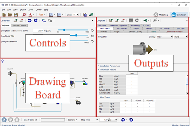
Figure 6‑1 – Three Regions of Simulation Mode (Controls, Outputs, Drawing Board)

Input controls are displayed on one or more tabs. You can create as many tabs as you like and organize the controllers in whatever way is convenient. For example, you can place all the file input controls in a single tab and controls for the optimizer independent variables in another.

Controls Toolbar

At the top of the Controls section of the main window is the Controls toolbar.  This gives you access to many features pertaining exclusively to the input controllers

Figure 6‑2 – Controls Toolbar

Here is a general overview of the buttons and their uses:

	New Tab – Controllers can be grouped together into tabs.  This button will create a new tab.
	Delete Tab – This will delete the current tab and its contents.
	Reset All Controls – This will reset all controllers on all tabs to their initial values.
	Input Control Properties – See the Input Controls Properties section below.
	Transfer Values to Layout – See the Transfer Controller Values section below.
	Transfer Controls to Scenario – See the Transfer Controller Values section below.
	Tab Listing – This displays a drop-down list of all the control tabs so that you can easily select the desired one.  This can be useful when you have many tabs.

Types of Input Controls

There are two main types of input controllers:

· Direct (user interactive) controls

· Indirect (program-mediated) controls

Each of these control types is discussed in the next section.

Direct Controls

Direct controls are those that you can set up and change interactively as the simulation proceeds.

There are three types of direct controls that you can set up in GPS-X (Figure 6‑3):

1. Slider Control: The slider control sets the value of the independent variable and gives a visual indication of the setting and a text display of the current value. You must specify a minimum and maximum for the slider control.

2. Increment Control: This control consists of two buttons, which add or subtract a specified amount to the current value of the independent variable. You must specify the increment, minimum and maximum for this control. Three system-defined controls that set the simulation stopping time, communication interval, and delay make use of increment controls.

3. Discrete Control: One type of discrete control is an on/off (2-state) button, which allows you to activate or de-activate an independent variable. For multi-valued text variables, this control is displayed as a pull-down menu of mutually exclusive buttons. Pressing one of these buttons causes the others to pop-up.

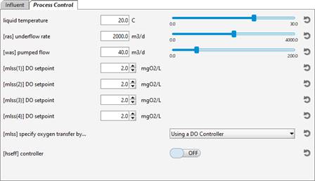
Figure 6‑3 – Example of Different Types of Input Controls

With the slider or increment type controls, you can type in the value on the line to the left of the slider or buttons. When you press the Enter key after typing in the value, the new entry will take effect. In the case of the slider control you will see the slider pointer move to the new position. If you enter a value outside the bounds of the min/max, the number will change to red to alert you, but the value is still used as is.

The slider, up/down, ON/OFF and pull-down menu controls have a “reset” button located at the far right of the control.  Pressing this button will reset the controller to the default value (taken from either the layout or the current scenario).

Indirect Controllers

The idea of a control extends beyond that of user-interactive control of an independent variable to include control of variable(s) by routines within GPS-X itself. These routines include:

· File Input Control: This function reads data from files. This data might be generated by other simulations, produced with spreadsheet or word processing programs, or collected from an actual plant. The data can be continuous, for example values of the influent flow rate, or they can be discrete, for example, ‘on’ or ‘off’ and ‘option 1’, ‘option 2’, etc. See the Using File Input Controllers section of this chapter for more information about setting up and using this feature.

· Analyze Control: These routines automatically vary the value of an independent variable. You specify the minimum, maximum, and an increment, and GPS-X runs the appropriate number of simulations to generate the sensitivity analysis results. There are additional input data requirements for sensitivity analysis. More information on setting up and performing sensitivity analysis is given in CHAPTER 9.

· Optimize Control: These routines calculate the optimal value of variables using specialized procedures to obtain targeted results. More information on setting up and performing an optimization is given in CHAPTER 10.

For each of these control types, you provide certain initial set-up information. GPS‑X then controls, or sets, the value of the independent variable accordingly. The graphical objects displayed for each of these control types is a non-interactive gauge, which indicates the current value.

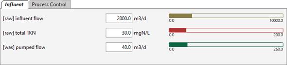
Figure 6‑4 – Indirect Control Types – File Input (Yellow), Analyze (Red) and Optimize (Green)

Creating A Control From An Independent Variable

Specification of the independent variables for which you would like to prepare a control is done by dragging the desired parameter to an input control tab from a data entry menu (Figure 6‑5).

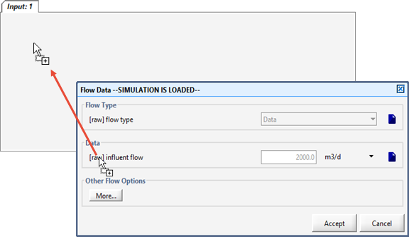
Figure 6‑5 – Dragging Variable to Control Tab

To access the data entry menu, right-click on an object to display the process data menu for the object of interest and select the appropriate independent variable menu item as demonstrated in Figure 6‑6.  Data entry menus are accessed by selecting either the Flow or Compositionmenu items for influent objects or the Input Parameters or Initial Conditions menu items for other process objects.

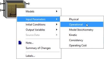
Figure 6‑6 – Example of Process Data Menu

Some parameters in the data entry forms are unable to be dragged to an input control window because these variables cannot be changed as the simulation proceeds. These include variables that would require a recompilation of the model, such as the number of reactors in series in a plug flow reactor.

It is important to differentiate between setting up input controls and setting up output display graphs as described in the next chapter. The procedure for both is similar; however, the selection of display variables is made only from the Output Variables menu item for a process object.

Quick Tip:  You can quickly create new input control tab by dragging a parameter (from a menu or another input control window) to the blank area to the right of existing tabs.  By doing so, a new tab will be created, and the parameter assigned to it.  This eliminates the need for clicking on the “New Tab” button first.

Input Controls Properties

Once you have created one or more control tabs and filled them with parameters to be used as interactive controls, you can then specify the properties of the controls themselves.

Clicking the Input Controls Properties… button (Figure 6‑7) will bring up the Control Properties dialog. 

Figure 6‑7 – Accessing Input Control Properties

In this dialog window, you can specify the units, ranges, and types of controllers for each input control parameter, as shown in Figure 6‑8.

There are several different options for the type of controller, including:

1. Slider

2. Up/Down (increment)

3. On/Off (discrete variables only)

4. Analyze (Step & Monte Carlo)

5. Optimize

6. File Input

Note: Some options may not be available depending on the specific variable

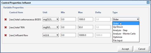
Figure 6‑8 – Input Control Properties showing Control Type Options

The interpretation of minimum (Min), maximum (Max), and increment (Delta) values is different for each type of control as described below.

· Slider Control: The minimum and maximum values define the total range of the slider. The resolution of the slider is 1/100th of the range calculated as maximum value - minimum value. The value of delta is ignored.

· Up/Down (increment) Control: The minimum and maximum values define the range over which the variable can be incremented. The value of delta is taken as the increment value.

· On/Off (discrete) Control: For this control, there are discrete choices (two or more). Values for minimum, maximum, and delta are ignored.

· Analyze Control: The minimum and maximum values define the limits of the analysis. For more information about analyze control, see CHAPTER 9.

o In a step sensitivity analysis, the independent variable varies from the minimum value to the maximum value in increments of delta.

o In a Monte Carlo analysis, the independent variable varies randomly within the range following the defined probability function

· Optimize Control: The minimum and maximum values are used as constraints in the optimization procedure. The optimizer will not set the independent variable to a value less than the minimum nor greater than the maximum. The delta value is ignored. For more information about optimize control, see CHAPTER 10.

· File Input Control: The minimum and maximum values are used to filter the input data. When a datum is read, it is compared with these values. If the input datum is less than the minimum, then it is set equal to the minimum value. If the input datum is greater than the maximum, then it is set equal to the maximum value. The delta value is ignored. For more information about file input controls, see the Using File Input Controllers section of this chapter.

Renaming an Input Control Tab

The name of an input control tab can be changed by simply double-clicking on the tab name, changing the text, and pressing ‘Enter.’

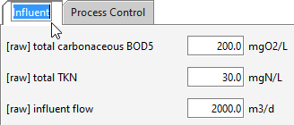
Figure 6‑9 – Renaming a Control Tab (Method 1)

Alternatively, right-clicking anywhere on the tab (other than parameter names) and selecting “Rename Tab” will bring up the window shown below:

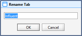
Figure 6‑10 – Renaming a Control Tab (Method 2)

Removing a Control

To remove a variable from an Input Control tab, right click on the parameter name, and select “Remove Input Control”, as shown in Figure 6‑11.

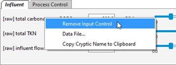
Figure 6‑11 – Removing an Input Control (Method 1)

You can also remove the controller by accessing the “Input Control Properties…” dialog window and clicking on the red ‘x’ beside the variable (Figure 6‑12).

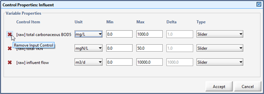
Figure 6‑12 – Removing an Input Control (Method 2)

Transfer Controller Values

There are times when you may have used the controllers to fine-tune a calibration of your model and once you are satisfied with the results, you’d like to use those values as the default values for either your layout or a scenario (for information on scenarios, see the section Using Scenarios in CHAPTER 8).

To accomplish this, we have added two buttons to the Controls toolbar to simplify this task.

Transfer Values to Layout

This feature will give you the option of selecting (from the current tab) which control values you would like to transfer and use as the default values of your layout.  Transferring values to the layout will cause the layout to be saved and the model to be rebuilt with the new values.

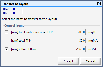
Figure 6‑13 – Transfer to Layout

Transfer Controls to Scenario

This feature is only enabled if a scenario has been selected (see Using Scenarios).  It will give you the option of selecting (from the current tab) which control values you would like to transfer and use in the scenario.  As opposed to transferring the values to the layout, this action does not require for the model to be rebuilt. 

Using File Input Controllers

In many cases, it is desirable to use data generated outside of GPS-X as input to the simulation model.

For example, it might be convenient to use actual plant influent flow and composition data as input to the model to observe the difference in response between the plant effluent data and model predictions. Operational reports, such as those recording a step-feed strategy, might be used to set up a file containing instructions on how to change the model to mimic the operation in the real plant.

The File Input control type reads data directly from a properly formatted ASCII or Excel file.

There are two methods for preparing data for a File Input controller: manually preparing data files, and using the GPS-X data file editor.

Manually Preparing Data Files

Any number of data files (in standard ASCII text or Excel spreadsheets) can be read and used as model inputs (input excitations or driving functions) or for display in GPS-X.

While the files can reside anywhere on your computer, it is suggested that you place them in the same directory as the layout files or a subdirectory of that location.

ASCII Text Files

For ASCII text files, you will need to know the cryptic variable name and the time-stamped data values.   The file must be saved with the extension .dat or .txt.

The format for this file is as follows:

t<delim>cryptic-name-1<delim>cryptic-name-2<delim>...

unit<delim>unit<delim>unit...

time<delim>data-1<delim>data-2...

.

.

.

The first line in the file is a tab or space delimited header containing the identifier ‘t’ (for time) followed by the cryptic names for the independent variables.

The second line specifies the units that the data is expressed in (columns are separated by delimiters).

Subsequent lines must contain the time stamp, in decimal form and the data values (columns are separated by delimiters). 

An example of a data file for the variables bodcon and tkncon for the stream with a label of raw is shown below.

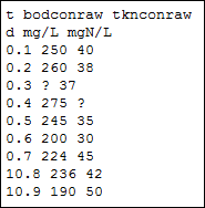
Figure 6‑14 – Example of ASCII Data File

Excel Data Files

Data files can also be prepared using Excel.  The format is similar to the ASCII text files, except that cells are used instead of delimiters to separate the data.

The first row in Excel is the header line that contains the cryptic names for the variables. Time (‘t’) is the first column.

The second row specifies the units that the data is expressed in.

Subsequent rows must contain the time stamp, in decimal form and the data values.

An example of a data file for the variables bodcon and tkncon for the stream with a label of raw is shown below.

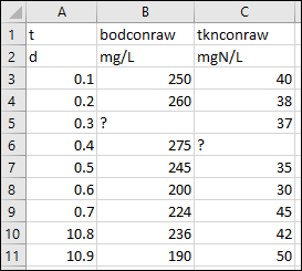
Figure 6‑15 – Example of an Excel Data File

New Data File Creation Tool

A tool has been included in GPS-X to simplify manual data entry in Excel by creating an Excel template file where the first two rows of data are populated by GPS-X.

To access the New Data File Creation tool:

	(1) Open the Data File Menu. On the main toolbar press the Data File button to open the Data Files window.
	(2) Create a new Data File. Pressing the New button on the Data Files window will open the New Data File Creation window. This will allow you to create a new Excel template file to be applied to the current scenario (see Using Scenarios) The New Data File Creation Window can be seen in Figure 6‑16.
	(3) Choose the Type of Data File. There are two types of data file variable types available: · If the Input Variable option is selected, the variables available to add to the data file will be limited to the variables that currently have an input controller. The data entered in this file will change the value of the input controllers during the simulation. · If the Output Variable option is selected, the variables available to add to the data file will be limited to the variables that are currently on an output display. The data entered in this file will be displayed on the output graph to compare the simulation results to observed results (see CHAPTER 8).        Press Next.
	(4) Select the Variables. All the currently available variables will be grouped by the tab they are currently placed on in the options pane. Expand the tab name lists to select variables. When a variable is selected it will appear in the Current Selection pane. When all variable selections are made, press Next.
	(5) Save the File. By default, GPS-X will save the Excel file with the same name as the layout in the same directory. These defaults can be changed by pressing the Browse button. Press the Finish button to save the file. You will be prompted to open the template file after it has been saved.

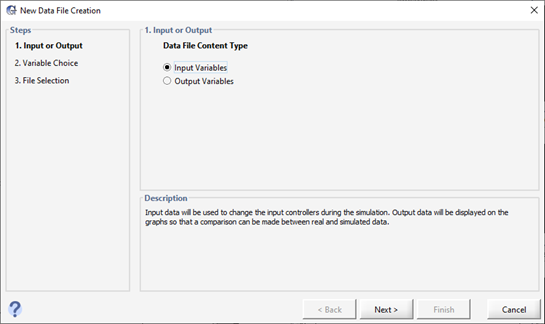
Figure 6‑16 – Using the New Data File Creation Tool

Special Characters

?	Fields in a data file that contain a question mark are interpreted as missing data.  In this case, the last valid data input for that variable is used.
std	If you enter a timestamp with the value ‘std’ that is interpreted as the value(s) to use at the start of a steady state simulation run.  As opposed to the value ‘0.0’ which is used at time zero.

Using the Data File Editor

GPS-X contains a simple tool for writing and editing .dat files (ie. ASCII text files with an extension of .dat).  This tool can only create/edit a file that will be used for a single variable, so its use is only suggested in simple cases or for beginners to GPS-X.  More advanced users typically prefer to edit their files externally to GPS-X so that they can include many variables into one file.

The editor can be accessed in several different ways:

(1) Through the Input Control Properties dialog.  When you change the desired controller to a file input type, a button will appear beside the Type box that will give you access to the editor.

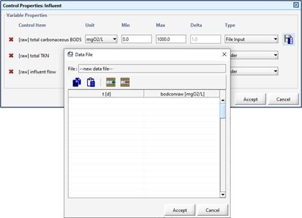
Figure 6‑17 – Accessing the Editor through the Control Properties Dialog

(2) Right-clicking on the controller label.  This will pop up a menu where “Data File…” is one of the options.

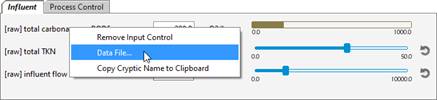
Figure 6‑18 – Accessing the Editor through the Pop-Up Menu

(3) Right-clicking on the label in the data entry form. This will pop up a menu where “Data File…” is one of the options.

Adding Input Files to a Layout

Once the data files have been set up properly you have to let GPS-X know that it should use these files during the simulation. 

If you created the file using the GPS-X Data File Editor or the New Data File Creation tool, it is automatically added to the layout.

However, if you manually created the files external to GPS-X, you need to explicitly let GPS-X know that they exist.  To do that:

(1) Access the “Scenario > Configuration” dialog window from the Simulation Toolbar (see Scenario Configuration in CHAPTER 8).

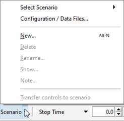
Figure 6‑19 – Add Files through Scenario Configuration

(2) From the list of scenarios (see Using Scenarios), choose the appropriate one and click the “Data Files” button.  This will display a dialog window with a listing of all the files that are currently being used by this scenario.

(3) From this dialog, you can choose to Add, Remove, or Edit a data file.

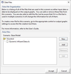
Figure 6‑20 – Add, Remove or Edit Data Files

Dynamic Data Validation

When manually creating a dynamic influent characterization data set, it can be time consuming to verify each set of influent conditions results in a valid influent characterization. To simplify this, GPS-X is equipped with a tool to automatically verify that each set of influent conditions creates a valid influent characterization.

To use the Dynamic Data Validation tool:

	(1) Open the influent advisor by right clicking on the Wastewater Influent object and navigating to Composition > Influent Characterization.
	(2) Open the Dynamic Data Validation tool by pressing the Dynamic Data Validation button in the bottom left corner of the influent advisor.
	(3) If you have manually prepared an influent data file, provide it to GPS-X by pressing the Browse button next to the Input File entry field. If you have not yet created an influent data file, press the Create Template button to have GPS-X provide you with a list of all the variables in the influent advisor. Select the variables that you have data for, and press accept. Save the file and populate it with data.
	(4) Create an Output File. Pressing the Browse button next to the Output File data entry field will prompt you to save a new file that GPS-X has created. This file is where GPS-X will write the results of the Dynamic Data Validation.

The Dynamic Data Validation tool will apply the influent conditions described in your input file to the influent advisor at each time step. The values calculated by the influent advisor at each time step will be written to the output file. You will be prompted to open the output file once GPS-X has completed the Dynamic Data Validation.

In the output file any conditions that result in an influent advisor variable taking a negative value will result in those conditions being highlighted yellow. GPS-X will also highlight the negative values in that row red.

Previous Next