CHAPTER 5
Introduction
You can create secondary variables that are calculated from existing model variables. Model variables are referred to as primary variables[3].
The Define feature is provided to make it easy for you to specify common secondary variables. You can add other calculated variables by modifying the model code directly. For more information on this topic, see CHAPTER 11.
You can specify daily and/or moving averages and mass flows for any variable in the model. This includes secondary variables that you may have defined previously, either in the code (CHAPTER 11) or with the define feature.
For example, with the define feature you can specify a secondary variable which contains the value of the moving average of the plant food-to-microorganism ratio.
Food-to-microorganism and solids retention time variables are special because normally they are calculated from primary variables at different locations in the plant.
For example, solids retention times can be calculated for a single treatment train, two or more treatment trains or the entire plant[4]. You can include the effluent suspended solids in calculation of the solids retention time or choose to ignore the effect of effluent solids on the calculated value. Similarly, you can evaluate the F/M ratio for a single reactor or multiple reactors and specify which unit process mass values should be used in the calculation. With the Define feature, you can specify how these variables are calculated for your plant.
The Define feature can be accessed through the Tools menu on the main menu bar or the Define button on the main toolbar.
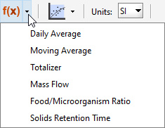
Figure 5‑1 – Define Menu Options
The types of variables that can be defined with this feature include:
For any model variable:
· Daily average
· Moving average
· Totalizer
· Mass flow
Or any layout:
· Food/Microorganisms ratio
· Solids retention time
Use the define feature during set-up of the layout, and before building the simulation model. You must always re-build the model after defining new variables.
Moving Averages, Mass Flows, and Totalizer
Moving averages, mass flows, and totalizers are often calculated for one or more variables in a treatment plant. The procedure for specifying these secondary variables is the same for all of them.
Moving Averages
Moving averages are data filters that smooth-out high frequency (rapid) changes in dynamic data so that it is easier to see overall trends.
Mass Flows
Mass flows are used in loading and material balance calculations.
Totalizer
This function will integrate the selected variable starting from time zero. The most typical application is integrating flow that is calculating the total liquid volume passed through the selected pipe during the duration of the simulation.
Concentrations totaled this way represent mass flow in a unit flow (1 m3/d) over the duration of the simulation. If the total mass flow (g/d) is required, it is best to use the Mass Flow function in the Define menu.
Follow this procedure to specify these secondary variables:
1. Click on the Define button and select either Daily Average, Moving Average, Mass Flows or Totalizer from the list (Figure 5‑1). A dialog window will appear as shown in Figure 5‑2.
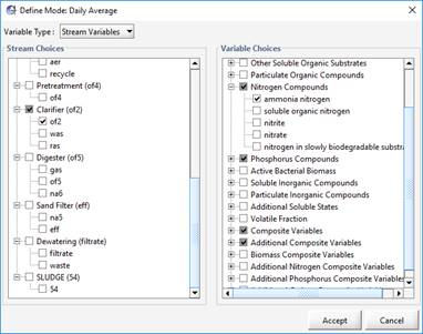
Figure 5‑2 – Define Dialog for Daily Average
2. Use the Variable Type drop-down box to change the display to the desired type of variable.
3. Select all the locations (left side) and variables (right side) to include in the calculation. Note that a checkbox with a grey background means that some, but not all the items in that grouping have been selected.
4. Click Accept to create the variable and close the dialog window
The secondary variables are now specified and are valid model variables like any other in the model. This means that you can display the defined variable, query the simulator for its value and include it in the definition of other secondary variables. For example, you might want to calculate the mass flow of solids into a reactor or clarifier and, from this, a moving average of the mass flow.
Specifying Moving Average’s Time Frame
After a moving average variable has been defined, the number of days to be used in the calculation can be specified in two different ways:
Through the Define dialog
(1) Open the Define dialog like you did to create the variable in the first place.
(2) Select “Define Variables” from the Variable Type drop-down box. A list of defined variables will be displayed.
(3) Find the variable of interest. Beside the variable will be an entry field where you can enter the number of days (Figure 5‑3).
(4) Click “Accept”.
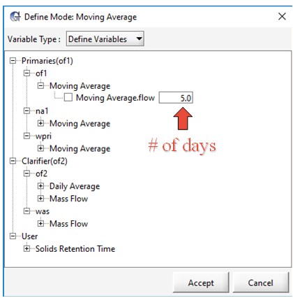
Figure 5‑3 – Specifying Moving Average Time Frame (Method 1)
Through the Process Data menu
(1) Right-click on the process that contains the defined variable. The process data menu will appear.
(2) Select Output Variables > Defined Variables > Moving Average. See Figure 5‑4. A dialog window with the defined variables will be displayed.
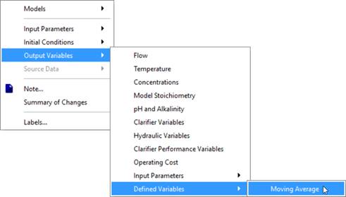
Figure 5‑4 – Viewing Defined Variables
(3) Enter the desired value into the entry field (Figure 5‑5)
(4) Hit “Accept”.
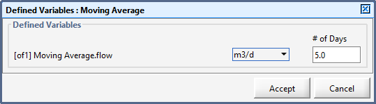
Figure 5‑5 – Specifying Moving Average Time Frame (Method 2)
The number of days that you set together with the communication interval specified for the simulation determines the number of points for calculation of the moving average. See CHAPTER 8 for information on simulation set-up including specification of the communication interval.
Remember that the communication interval defines the update frequency, and the number of days value defines the overall time window used in calculating the moving average.
For the daily (moving) average the time window is 24 hours and is calculated exactly regardless of the simulation communication interval. To calculate the daily average, GPS-X uses data obtained at each integration time step rather than the output communication interval.
Any defined variable becomes a normal, calculated model variable. You can display the variable and use the variable in other calculations; however, as it is a secondary variable you cannot set its value before or during a simulation run. Remember that you must re-build the model after defining new variables to display the calculated values.
Food/Microorganism (F/M) Ratio
The definition of food/microorganism ratio is often layout-dependent and, therefore, it is convenient to be able to define it differently for each layout you prepare. The procedure used to define the variable is interactive. Because it is based only on mass and flow measurements, the GPS-X define procedure has been designed to allow you to specify the form of the equation by simply clicking on the object or connection point containing the mass or flow value of interest.
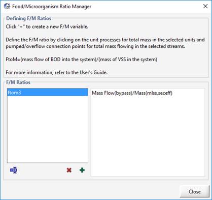
Figure 5‑6 – Food/Microorganism Ratio Manager
To define a Food/Microorganism Ratio secondary variable, complete the following steps:
|
|
1. Click on the Define button and select the Food/Microorganism Ratio item. The F/M Ratio Manager dialog window will appear (Figure 5‑6). |
|
|
2. Click on the “+” button to create a variable name for the new defined variable. The text area on the right side of the dialog displays the mass and mass flow terms used in the equation to calculate the selected variable on the left. You interactively specify the full form of the equation by clicking on objects and object connection points. |
|
|
3. Click on a unit process on the drawing board (not a connection point) to add that unit’s mass to the calculation of the mass term in the defining equation. When you move the cursor over an applicable unit process it will change the cursor to a hand. Clicking will add the object’s identifier label[5] as an argument in the Mass() term. If you click the same object a second time, the object’s identifier label is removed from the mass term. |
|
|
4. Click on connection points (not the object itself) corresponding to flow streams containing mass flow values of interest to add that connection point’s mass flow to the calculation of the mass flow term in the defining equation. When you move the cursor over an applicable connection point it will change the cursor to an arrow. Clicking will add the connection point’s flow stream label as an argument in the Mass Flow() term. If you click the same point a second time, the connection point’s stream label is removed from the mass flow term. |
|
|
5. After you have specified all appropriate mass and mass flow terms, click Close. |
Solids Retention Time (SRT)
The SRT Manager allows users to define multiple SRTs for a model layout. The SRT manger also allows the user to control sludge wastage via a SRT setpoint.
The SRT Manager can be used to define calculations for multiple SRTs if required. For example, it is possible to define aerobic SRT, anoxic SRT or anaerobic SRT by using the biomass in aerobic, anoxic, or anaerobic compartments, respectively.
To define an SRT secondary variable, complete the following steps:
|
|
1. Click on the Define button and select the Solids Retention Time item. The SRT Manager dialog window will appear. |
|
|
2. Click on the “+” button to create a variable name for the new defined variable. The text area on the right side of the dialog displays the mass and mass flow terms used in the equation to calculate the selected variable on the left. You interactively specify the full form of the equation by clicking on objects and object connection points. |
|
|
3. Click on a unit process on the drawing board (not a connection point) to add that unit’s mass to the calculation of the mass term in the defining equation. When you move the cursor over an applicable unit process it will change the cursor to a hand. Clicking will add the object’s identifier label[6] as an argument in the Mass() term. If you click the same object a second time, the object’s identifier label is removed from the mass term. |
|
|
4. Click on connection points (not the object itself) corresponding to flow streams containing mass flow values of interest to add that connection point’s mass flow to the calculation of the mass flow term in the defining equation. When you move the cursor over an applicable connection point it will change the cursor to an arrow. Clicking will add the connection point’s flow stream label as an argument in the Mass Flow() term. If you click the same point a second time, the connection point’s stream label is removed from the mass flow term. |
|
|
5. The “Estimate WAS using selected SRT” checkbox allows the user to estimate the waste flow rate for the selected SRT. Additional inputs like the SRT set point and min/max values for the calculated SRT controller pump flow are required. |
|
|
6. After you have specified all appropriate mass and mass flow terms, click Close. |
In the simulation mode, the values of the SRT can be visualized by dragging and dropping the SRT variables in the output window. The drag and drop action places both the instantaneous and dynamic SRT for visualization. Depending on the need, one or the other SRT can be removed from the outputs. In simulation mode, the SRT manager can also be used to turn off the WAS flow rate calculation based on SRT set point. The user can also change the set-point value in simulation mode.
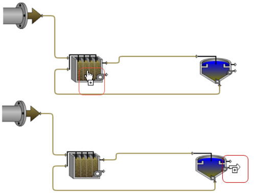
Figure 5‑7 – Selecting Processes/Streams for Defined Variables
Dynamic SRT
Under dynamic conditions the solids retention time (SRT) is based on an age balance performed on the sludge in a manner similar to a typical mass balance. At steady-state the dynamic SRT is equivalent to the SRT. In dynamically changing conditions the dynamic SRT gives a better approximation of the true age of the biosolids in the system and can replace empirical smoothing methods (seven day moving average, etc.) routinely used to filter the sudden fluctuations in the instantaneous SRT calculation.