Influents, flow control points (i.e. splitters and combiners), and unit processes are characterized by the data that define them. Here, the term data is used in a generic sense to refer to the values of all attributes that uniquely define an object. Foremost among these attributes are the models which describe the input-output behavior of the object. Some models are simple and require few parameters. For example, a two-way flow-splitter model has a single parameter – the fraction of the flow going to one of the two outputs (the other is calculated). Other models are complex, such as the biological nutrient removal models used in reactor objects. The kinds of parameters needed for an object depend entirely on the kind of model selected for that object.
Attributes can be classified as either numeric or text. Numeric attributes include parameters like the real dimensions of the unit (width, area, etc.) and kinetic constants (maximum specific growth rate, decay constant, etc.). Most of the attributes in GPS-X are numeric. Text variables include the type of model used to describe the object, the type of controller to use in a model, etc. Text variables have a discrete number of ‘values’. For example, the plug flow tank reactor can have only one of several types of models – one of the asm1, asm2, asm3, newgeneral, mantis2, or mantis3 models (not all of these models are available depending on which library you are using). Similarly, the controller type variable for the PID controller model can be P, PI, or PID. When specifying a value for a text variable, GPS-X provides a list of options from which to make a selection.
Every object placed on the drawing board must be fully specified before a plant model can be prepared. GPS-X simplifies this using default models and parameter values. In practice, it is often found that some model parameters do not change significantly[1], or do so within a certain range. Incorporating default values for model parameters in GPS-X minimizes the amount of data entry that must be done before a working model can be built. However, you must ensure that these values are appropriate for the particular plant or process being modeled.
Object data are specified by opening the appropriate data entry form and either making a selection from a list of options or entering numeric values. Data entry forms are accessed from the Process Data menus, which are defined for each object.
To display the process data menu:
1. Right click on any object on the drawing board. The process data menu for that object will be displayed.
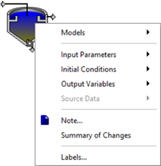
Figure 4‑1 shows the process data menu for the circular secondary clarifier object.
Figure 4‑1 – Process Data Menu for a Circular Secondary Clarifier
In GPS-X, one of the most important attributes of an object is the type of model used to simulate the input-output behavior of that object. Because of this, the first step in specifying object data is to select the model to be used for each object. This is done by selecting the Models item from the process data menu.
To specify a model type:
1. Pop up the Process Data menu by right clicking on any object on the drawing board.
2. Select the Models item. This will cause a hierarchical menu to be displayed as shown in Figure 4‑2.
3. Click on the desired model.
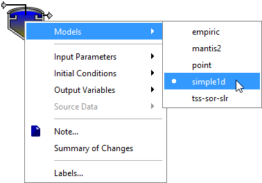
Figure 4‑2 – Selecting a Model
GPS-X automatically selects the default model for you when you first place the object on the drawing board. If you wish to switch to a different model, you will lose any parameters entered into the data menus.
If you wish to change the default model so that GPS-X will always choose your desired model, edit the defaultmodelchoice.txt file in the subdirectory bin/gpsx/resourcesin the GPS-X installation directory.
Not all objects have more than one model. For example, splitter and combiner objects have a single, pre-set default model so you do not need to make a model selection to access the parameters for these objects.
Once the model has been specified, you can access all the object’s attributes. These attributes differ depending on the model and type of object.
For detailed lists of object and model attributes, see the Technical Reference manual.
An object’s attributes are divided up into several categories.
Depending on the object type, the input variables are grouped into either:
(1) Composition and Flowif it is an influent object (see Influent Objects)
(2) or Input Parameters and Initial Conditions if it is any other object (see Process Objects).
The items under this group allow you to set the model characteristics in Modelling mode (see the Data Entry Forms section below) or select controller variables in Simulation mode (see CHAPTER 6 Preparing Input Controls).
The output group allows you access to all the variables that can be displayed on graphs or various other output displays in Simulation mode.
Allows you to specify (or remove) links to other unit processes where common data can be obtained. See the Sourcing section in this chapter for more details.
Allows you to make any personal notes about this specific object on the drawing board. These notes are purely for your own reference. They do not affect the layout in any way.
Allows you to see a summary of all the variables you have changed from their default GPS-X settings for a given object.
Allows you to view/edit the process and stream labels for this object (see the Labels section below).
For a complete description of the data entry forms and parameters for each model, refer to the Technical Reference manual. The following is a general description of the forms.
Data entry forms are displayed when you select one of the menu items under an input grouping (ie. Composition, Flow, Input Parameters, or Initial Conditions as described in the previous section).
Within each form, data are grouped into logical categories.
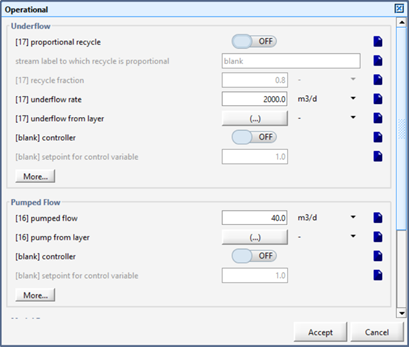
Figure 4‑3 – Data Entry Form Example for a Secondary Clarifier
In some cases, some of the less commonly adjusted parameters are grouped together on a separate data form, which is shown by the presence of a More… button.
Some parameters will appear “greyed-out” (ie. inactive). These are parameters that are only relevant when another parameter has been activated or selected. For example, when the proportional recycle is set to off, the recycle parameters will be inactive. This functionality is also tied to the drop-down menus.
When the mouse is held over a parameter name, a tooltip appears which shows the descriptive and cryptic names of the parameter.
The purpose of this tooltip is twofold.
(1) One is to provide the descriptive name as some of the longer descriptive names may be cut-off in the data entry form due to space limitations.
(2) The second purpose is to show the cryptic name of the parameter. Knowing the cryptic name of a parameter is sometimes needed for setting up controller models, or for adding customized model code. For more information on the conventions used for setting cryptic parameter names, see the Technical Reference manual.
To the right of the descriptive label for a parameter is an entry field for entering input. The entry field may be a data entry field, a text entry field, a drop-down menu from which a selection can be made, or an ON/OFF button. If the variable is an array, an Array button [(…)] is displayed. To access the individual array elements, click on the array button, and another form will be displayed for entering values in each element of the array.
When values are entered that are different than the default value, the new value will be shown in bolded blue text. The default value can still be viewed by holding the mouse cursor over the entry field to display the tooltip.
The unit of the input variable can be changed by clicking on the unit label.
|
To the right of the units is a button that allows you to add a note about each parameter. Once notes have been made, the button’s icon will change, and the note will appear as a tooltip pop-up when the mouse is held over the button. The notes function also supports the use of HTML tags. |
|
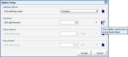
Figure 4‑4 – Data Entry Form Example (with Notes Field in use)
The composition, concentration, and flow characteristics of the influent are major factors determining the dynamic behavior in unit processes that make up the plant. GPS-X allows you to specify the type of flow or load pattern. You can specify a constant or sinusoidal flow or load pattern by entering only a few parameters in the Wastewater Influent object. You can enter a single diurnal pattern for GPS-X to repeat or you can enter your own flow and/or composition data and have GPS-X use these data for the influent. These attributes are entered by making selections from the Composition and Flow process data menu items.
The majority of an influent model’s attributes are accessed through the Composition item. These parameters have been further divided into categories depending on the specific type of influent (Continuous or Batch).
Influent Characterization accesses the Influent Advisor tool to aid in the setup of your influent object (see CHAPTER 3).
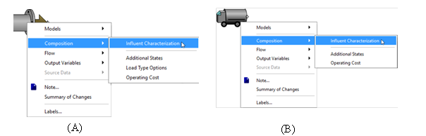
Figure 4‑5 – Influent Object Composition Menus for (A) Continuous and (B) Batch
NOTE: Not all influent models have all the menu items displayed in Figure 4‑5
The Flow > Flow Data item is used to enter a flow type and related data. The continuous wastewater influent object differs from the batch influent and chemical dosage objects in that it contains a specialized runoff model.
A variety of parameters are needed to specify a unit process; however, these can be categorized as either input parameter or initial condition values. Input parameters include physical, kinetic, operational and stoichiometric data, whereas, initial condition values refer to initial conditions for the model state variables including the volume and component concentrations.
The majority of a model’s attributes are accessed through the Input Parameters item. These parameters have been further divided into categories depending on the specific type of object.
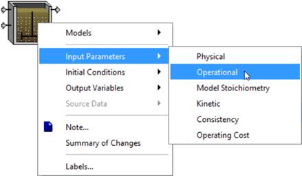
Figure 4‑6 – Input Parameters Sub-Menu Example
Initial conditions are defined only for non-point process objects; that is, objects which have a volume. Point process objects include objects such as flow splitters and combiners, which are modeled as zero-volume control points. Point objects do not require initialization because there is no accumulation or utilization of material within the object. Point objects serve only to distribute or collect flows coming into the object.
In practice, initial conditions are rarely set manually unless data are available from previous simulations and you want to restore these conditions before re-starting the simulation, or if you are interested in starting the simulation with certain initial volumes (for example, with one or more tanks partially full). In the majority of cases, the default initial conditions – which are pre-defined for the model’s default data – are used. For a given set of initial conditions, the usual procedure is to first run the steady-state solver to determine a valid steady-state, and then run a simulation. Alternatively, you can run the simulation for a period (i.e. 1 day), save the state variables, reinitialize the state variables and then conduct a simulation. See Initial Conditions in CHAPTER 8 for more information on setting the initial conditions for a simulation run.
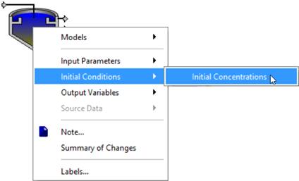
Figure 4‑7 – Initial Conditions Sub-Menu Example
When constructing a model in GPS-X, the default settings for each variable provides a good starting point for most applications, but you will often need to modify these defaults to match your plant characterization and performance. For large models that are highly customized, it can be difficult to track all the changes that have been made to the GPS-X default settings. In Modelling Mode, the Summary of Changes menu item can be used to provide you with a quick summary of each variable in an object that the user has changed from its GPS-X default value. The Summary of Changes from the Default results for a wastewater influent object can be seen in Figure 4‑8.
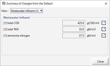
Figure 4‑8 - Summary of Changes for an Influent Object
The name and current value of each modified variable for the selected object appears in the Summary of Changes output. Beside each variable value is a Go to location button which will take you to that variables data entry form where you can further manipulate the variable or reset its value to the GPS-X default value.
The View drop-down menu at the top of the output can be used to navigate between the objects on the layout. A Summary of Changes output will be available for each object that is currently placed on the drawing board.
Among the important system-related attributes of every
object in a GPS-X layout are the connection point labels for that
object. When you drop an object icon on the drawing board,
GPS-X assigns a numbered label to each connection point in that
object. The label is used to generate model variable names, develop
the model equations, and manage the changes, which occur in each
variable. These processes are transparent and need not interfere
with the process analysis tasks you perform. In fact, a key
advantage of GPS-X is its ability to hide lower levels of
complexity so that you can concentrate your efforts on process
analysis and understanding.
In some cases, it is necessary or convenient to determine or possibly change the labels assigned to connection points on an object. To do this, you can use the Labels… item in the process data menu.
To change the labels on an object, complete the following steps:
1. Right click on an object. Select the Labels… item. This will cause the label dialog box to be displayed.
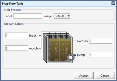
Figure 4‑9 – Labels Dialog
2. Enter any alphanumeric string at each connection point. You can enter any string you like. The only constraint is that if the label consists of more than one alphanumeric character, the name must begin with a letter, not a number. For example, the labels a, 1, and a1 are acceptable, but 1a is not. GPS-X will not allow you to enter invalid strings (i.e. spaces are not allowed and certain characters cannot be used to start a string). The label can be up to 31 characters in length.
3. Enter any alphanumeric string in the ‘label’ text box. This is the process’s label and is displayed above the object on the drawing board. It can also be useful for differentiating between objects when the output displays are created.
4. Click the Accept button to save these values. If you entered a label that is already in use, an error will be displayed, and you won’t be able to ‘accept’ the changes until the duplications are corrected.
The connection point labels are used as flow stream identifiers and to generate variable names (referred to as ‘cryptic’ names) in the dynamic process model. Cryptic names are created by taking a default descriptor, such as ‘muh’ for heterotrophic maximum specific growth rate and appending the label to that descriptor.
For example, the cryptic variable containing the value of soluble BOD for an object’s influent labeled ‘inf’ is ‘sbodinf’.
By convention, any variables internal to non-point objects take the output connection point label when constructing the variable name.
As an example, if a continuous flow stirred tank reactor has ‘140’ as the label for the output connection point, the heterotrophic maximum specific growth rate (descriptor ‘muh’) in the reactor would be named ‘muh140’.
There are two ways to view the cryptic names.
(1) For individual parameters, position the mouse over the variable label of interest whereby a tooltip will appear with the descriptive label and the cryptic name separated by a back slash. See example in figure below.
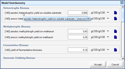
Figure 4‑10 – Viewing the Cryptic Name via Tooltip
(2) Another way to view the cryptic names is by selecting the Show cryptic variable names option in View > Preferences > Layout tab under the Display group.
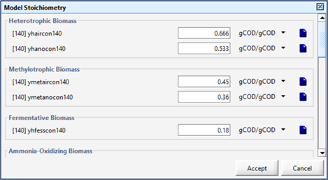
Figure 4‑11 – Viewing the Cryptic Names via Preferences Setting
This will change it so that the cryptic name is shown in all data entry forms instead of the descriptive label. This can be confusing, so it is recommended that the cryptic option be used with care. The data entry label names will be refreshed each time you accept the changes to the Preferences menu.
For more information on model variable names and conventions used in constructing these names, please see the Technical Reference.
By default, labels are not displayed on the GPS-X drawing board[2]. If you would like to have them displayed, use the Label drop down menu on the Toolbar and choose either ‘streams’, ‘objects’ or both.
Figure 4‑12 – Layout Before and After Displaying Process/Stream Labels
Labeling procedures in GPS-X are important when you need to uniquely identify an object and/or its streams. This is the case when object data are linked together as discussed in the Sourcing section of this chapter.
When you are constructing a model, there may be times where you wish to modify, control or visualize a variable but you are unsure of which menu it is located in. If you know part of the variable’s common name or have a cryptic variable name from a GPS-X output, the Find function can be used to locate the menu.
To open the Find window, go to Edit > Find to open the data entry window for the find functionality, as seen in Figure 4‑13.
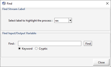
Figure 4‑13 - Find Menu Entry Form
In the Find Stream Label section of the Find Window is a drop down which contains all the stream labels on the layout. Selecting a stream label from this drop-down menu will highlight the object in the layout that the stream originates from. This can be used to identify the object that unfamiliar model outputs originate from.
The Find Input/Output Variable section of the Find menu is used to locate variables in GPS-X. If you are unsure of the variable you are looking for, keywords you expect to be in the variable name can be entered into the Find entry field with the Keyword toggle selected. For example, entering ‘underflow’ into the find entry and pressing the Find button will yield the results seen in Figure 4‑14.
Using the find function will give you a list of all the
variables that contain the keyword ‘underflow’. The variables will
be organized by both the object they are associated with on the
GPS-X layout and if they are an input or an output variable. If you
press the “Go To Location” ![]() next to the variable name it will take you
to the menu where the variable is defined. If the variable is an
input, you will be taken to a data entry menu, while an output
variable will take you to a display variable menu.
next to the variable name it will take you
to the menu where the variable is defined. If the variable is an
input, you will be taken to a data entry menu, while an output
variable will take you to a display variable menu.
Alternatively, if the cryptic variable name is known, the Find function can be used to find all variables whose cryptic variable name contain the known cryptic variable name. To search a cryptic variable name, enter it in the data entry field in the Find Input/Output Variable section of the Find menu and toggle on the Cryptic option below the entry field. Press the Find button and GPS-X will display all instances of the cryptic variable in the layout, formatted the same way as the Keyword find results.
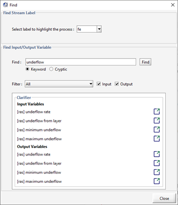
Figure 4‑14 - Find Results for Underflow
Data entry is an important aspect of building and maintaining a dynamic process model. Once the model structure is in place, it is necessary to identify those parameters which are most important and then determine how to adjust these to obtain the desired model behavior. With conventional modelling and simulation software this task consumes a large fraction of the model development time, using resources that could be more profitably applied elsewhere. One time saving feature is specifying Source objects.
In GPS-X, attributes are linked to specific objects. This linkage mechanism is a simple way to reference objects to their data and makes it possible to link multiple objects to a single data set. When one object (a parent), becomes a source for a second object (a child), the latter inherits data from the former. This is the essence of the concept sourcing in GPS-X.
The real power of sourcing becomes evident when changes are made to object data, for example, due to model calibration, on-line data entry, etc. When objects are properly sourced, this change need only be made in one place – at the source object. If the sourcing feature was not used, these changes would have to be made for each appropriate object affected by the change.
NOTE: Not all data are inherited. Only the kinetic and stoichiometric parameters for reactor models and settling parameters for sedimentation models are inherited. The same model type must be selected for both objects before any sourcing links can be established.
Note the following constraints when sourcing:
· Sourcing of kinetic and stoichiometric parameters can only be established between objects with the same model type.
· Sourcing specifications cannot include inheritance loops, that is, you cannot specify a data chain of sourcing relations in which a parent object inherits from one of its child objects. It is not possible to determine a unique parent object in a sourcing chain forming a loop.
· Biological reaction unit processes can inherit kinetic and stoichiometric parameter values from any other biological reaction unit process with the same model.
· Sedimentation unit processes can inherit settling parameters from other sedimentation unit processes of the same kind. Secondary sedimentation and sequencing batch reactor objects can inherit from other secondary sedimentation or sequencing batch reactor. Sedimentation unit processes which have reactive models can inherit kinetic and stoichiometric parameter values from any other biological reaction unit process.
To specify a source object (parent) for another object (child) of the same type:
1. Right-click on the child object. The process data menu for that object will appear.
2. Highlight the Source Data option (Figure 4‑16). If that option is disabled (greyed out) then that means that there are no potential data sources (ie. parents) currently on the layout.
3. Select the parent object from the list. The child will now automatically inherit data from the parent.
NOTE: A ‘chain’ icon will appear on the child object’s image on the drawing board to easily identify which processes have been sourced (Figure 4‑17).

Figure 4‑15 – Example Layout before adding Source Links
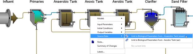
Figure 4‑16 – Example Layout showing Source Data menu
Figure 4‑17 – Example Layout showing Source Linked Processes
To remove (or view) the current source of an object, complete the following steps:
1. Right-click on the child object to display the process data menu.
2. Highlight the Source Data option. The sub-menu will display other potential parents (if applicable) and below that is the option to remove the current parent.
There are some data which are not exclusively related to influent, process, or flow path objects. This includes operating system and simulator module set-up information, such as timing parameters, numerical integration options, and process environment parameters such as temperature. The data entry forms for this data are accessed from the Layout menu on the main menu bar. It can also be accessed by right-clicking on a blank area of the drawing board.
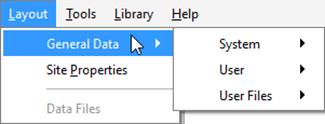
Figure 4‑18 – General Data Menu
The System menu is used to gain access to the global simulation parameters, such as parameters related to the operation of the steady-state solver and the optimizer.
The User menu is used to gain access to the user-defined variables. This item is provided for advanced users to customize the GPS-X interface. The user can define any number of additional parameters or initialization and display variables, and then access these here. For more information on customizing GPS-X see CHAPTER 11.
The User Files menu is used to define custom code and user-defined variables. This item is used to access the GPS-X user-customizable files, which give users the ability to define, use and display customized user code. For more information on customizing GPS-X see CHAPTER 11.
The Site Properties item is merely a subset of the most commonly used data in the General Data category described above.
It allows users to customize the physical input parameters of the plant (Plant Site Properties tab) and the simulation date (Simulation Setup tab). Additional plant information notes can also be saved under the Plant Information tab.