CHAPTER 14
Introduction
Model Developer is a utility that allows GPS-X users to create and edit their own models in GPS-X. Model Developer makes use of the model matrix format for model specification, which is the standard format in the wastewater modelling literature. For more information on model matrix notation, please consult the IWA report on the structure of the ASM1 and ASM2d activated sludge models (Henze, et al., 1987, and Henze et al., 1998, respectively).
This chapter provides instruction on how to use Model Developer (MD), and assumes the user is familiar with mechanistic dynamic activated sludge models, and matrix notation format.
As the MD tool creates and edits files within the GPS-X directory, read and write privileges in the GPS-X instillation directory are required. Ensure you have the appropriate privileges before using MD. Depending on where GPS-X is installed on your machine, GPS-X may need to be opened in administrative mode or reinstalling in a different directory on your machine to get the appropriate privileges to use MD.
Accessing Model Developer
The MD tool is an interactive utility for creating and editing models in GPS-X. To access model developer, navigate to Tools > Model Developer on the main toolbar.
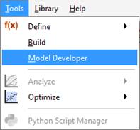
Figure 14‑1 – Accessing the model developer
Model Developer Components
MD is an application within GPS-X that organizes model content into a series of pages that contain information on model structure, parameters, and GPS-X variables. These pages are used, along with templates found in each GPS-X library, to create a biological model written for the following GPS-X unit process objects:
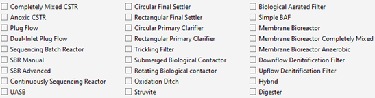
Figure 14‑2 – GPS-X Object Biological Templates
In each case, the biological model is implemented with the appropriate physical characteristics and hydraulic configuration for the given object.
There are 5 sections to the Model Developer Tool, accessible through tabs at the top of the model developer window: GPS-X Libraries, Stoichiometric Matrix, Model Kinetics, Model Parameters, and Composite Variables.
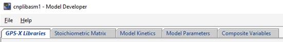
Figure 14‑3 – Sections of Model Developer
GPS-X Libraries
The GPS-X Libraries page shows information on the existing set of state variables and composite variable stoichiometry parameters in the GPS-X libraries, as well as the library-specific composite variable calculations. These are not changeable. Models can be made up of a full set or subset of the state variables shown on these pages. Select the appropriate library (from the Library: pull down menu) to display the state variable and composite stoichiometry set, and composite variable calculations.
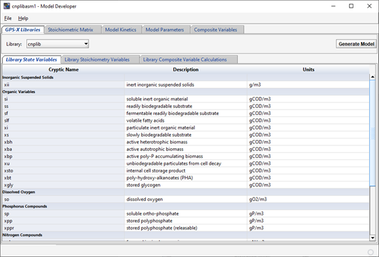
Figure 14‑4 – State Variables and Composite Stoichiometry in the cnplib Library Tab
Stoichiometric Matrix
The Stoichiometric Matrix tab shows the model matrix for all models available. You can select the appropriate model from the Model Name: drop down menu.
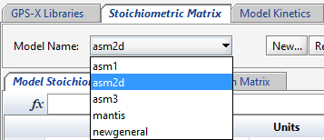
Figure 14‑5 – Stoichiometric Matrix Selection
The Model Stoichiometry tab shows the model matrix, with state variables in columns and kinetic processes in rows. Textual descriptions of the kinetic processes are shown on the left.
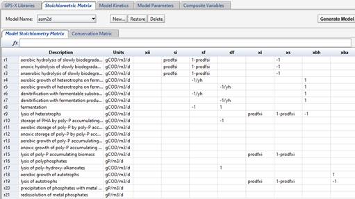
Figure 14‑6 - The ASM2d Model Stoichiometry Matric
The Conservation Matrix tab shows the elements of the conservation matrix, used to calculate unknown model stoichiometry via mass balance. For more information on using conservation matrices, please see the ASM2d report. The element in the model stoichiometry table that will be calculated from the conservation matrix is filled with the symbol @{var}, where {var} represents the element being conserved, as shown in the left column of the conservation matrix (e.g. @COD).
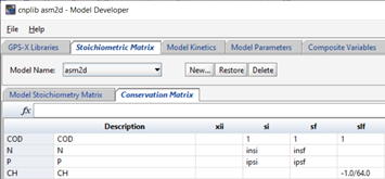
Figure 14‑7 - The ASM2d Conservation Matrix
Model Kinetics
The Model Kinetics page contains information on the kinetic process rates used in the model (which are represented by rows in the model stoichiometry matrix). The Saturation/Inhibition Functions tab shows all saturation and inhibition functions used in the creation of the kinetic process rates. Each variable is shown with its corresponding equation and units.
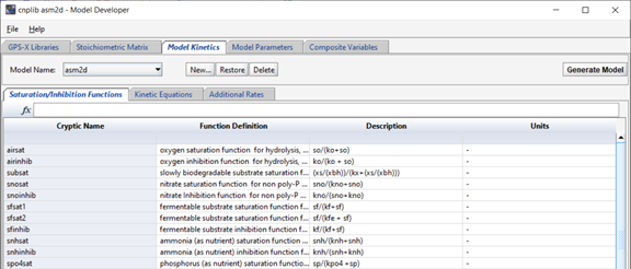
Figure 14‑8- Saturation and Inhibition Functions used in the ASM2d Model Kinetics
The “Kinetic Equations” tab shows the kinetic equations themselves. The rates and descriptions match those shown on the model stoichiometry tab. The corresponding rate equations and units are shown and edited on this tab. If new rates are added to the stoichiometric matrix, new corresponding rows will show here as well. Any saturation functions that should be applied to the kinetic rates in the biofilm objects (only) can be selected from the drop-down menus in the right-hand column.
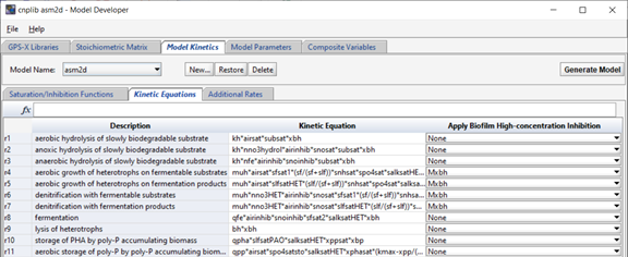
Figure 14‑9 - Kinetic Equations in the ASM2d Model
Any other additional equations that might be useful to calculate in all reactors can be added in the “Additional Rates” tab.
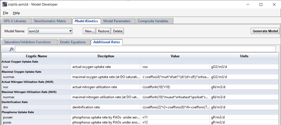
Figure 14‑10 - Additional Equations in the ASM2d Model
Model Parameters
The fourth tab of the MD tool (labelled “Model Parameters”) contains variables and parameters that are part of the model. Each variable/parameter is listed along with its descriptive name, value, and appropriate units. This page includes:
· State Variables:the model state variables, and their initial values, and diffusion coefficients for biofilm objects.
· Stoichiometric parameters: both model stoichiometric parameters (from the Model Matrix, such as yield, etc.) and organic/nutrient fractions are listed here (e.g. N fraction of biomass).
· Kinetic parameters: model kinetic parameters are listed here, including values for 10 C and 20 C temperatures, or Arrhenius temperature coefficient.
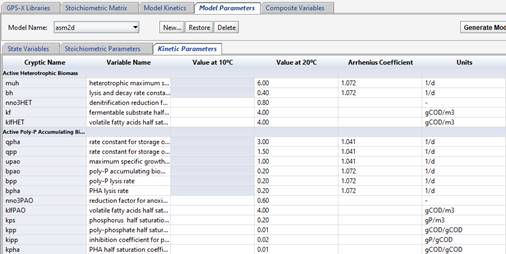
Figure 14‑11 - Model Kinetic Parameters of the ASM2d Model
Note that if temperatures are entered for both 10 C and 20 C, the Arrhenius coefficient will be calculated from these values. Alternatively, you can enter just the 20 C value, and enter an Arrhenius coefficient directly.
Composite Variables
The final tab on the MD page is the Composite Variable page, where the stoichiometry of the model is assigned to the fixed GPS-X composite variable stoichiometry. For example, GPS-X has a fixed variable name for the nitrogen fraction of particulate inert COD – inxi. These variable names and descriptions are shown in the first two columns and are not changeable. If your model uses these model conventions, then you can select the appropriate value in the right-hand column. If you have nutrient fractions that are differently named than the fixed GPS-X variable set in the left column, then please select the appropriate variable name from the list. If you do not have an equivalent variable in your model for some of the standard GPS-X variables, you can set the GPS-X variables to zero.
Entering Models into Model Developer
The following 5 GPS-X activated sludge models are available in MD by default.
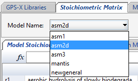
Figure 14‑12 - Default Active Sludge Models in Model Developer
To create a new model, select File > Save Model As… and save the model with a new name in the c:/gps-x85/md/models/ folder.
You cannot generate models that have the same name as an existing model in GPS-X – if you wish to regenerate a new, modified version of asm1 (for instance), you will have to give it a new name. This is done to protect the existing library structure.
There are 3 steps involved in preparing a model in MD:
1. Entering/editing the model stoichiometric matrix.
2. Writing the kinetic rate equations (including any internal saturation/inhibition functions) and any other supplemental kinetic rate equations of interest
3. Entering model parameters and default values
Specifying the Model in the Model Stoichiometric Matrix
The model matrix is specified in Model Stoichiometry page. New state variables may be added to the model (provided they are part of the GPS-X library) by right-clicking on a column and selecting a new state variable from the available list. New rates are added by right-clicking on the matrix and adding a new row.
Model stoichiometric relationships can be entered directly into each cell of the matrix by clicking on the appropriate cell and entering in the equation. Include a decimal place with all real values (including integers), when entering stoichiometric equations. Please note that MD does not support using commas for decimals points.
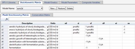
Figure 14‑13 – ASM2d Model Stoichiometry Matrix
The conservation matrix (shown on the conservation matrix tab) may be incorporated by entering values in the matrix that indicate which conservation element is used. For details of using a conservation matrix, please refer to the ASM2d model publication (Henze, et al., 1998).
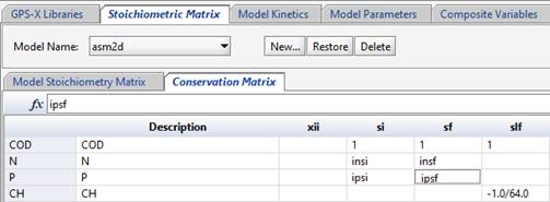
Figure 14‑14 - ASM2d Conservation Matrix
The nomenclature to be used in the cell for which the stoichiometry is to be calculated is shown below:
@COD – stoichiometric constant for the current row, based on COD conservation
Each stoichiometric constant that is determined from the conservation matrix must use only one of the conservation elements available (e.g. COD, above). Each conservation element is listed in a separate row in the conservation matrix and contains the appropriate stoichiometry for each state variable. For a good example of the use of the conservation matrix, please see the ASM2d model in MD.
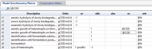
Figure 14‑15 - Identifying Stoichiometry COD Conservation in ASM2d
Entering Kinetic Rate Equations
On the Model Kinetics page, on the Kinetic Equations tab, the kinetic rate equations for each row of the matrix are shown. The descriptive name of the rate is shown here as well, along with the units.
If the rate equation contains terms that would be useful to have calculated separately (such as inhibition or saturation functions), those can be listed (along with descriptive names) in the “Saturation/Inhibition Functions” tab.
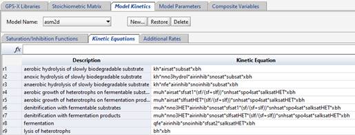
Figure 14‑16 - ASM2d Model Kinetics
The “Apply Biofilm High-Concentration Inhibition” term on the right-hand side is a feature that allows a saturation term (which must first be defined on the Saturation/Inhibition Functions tab) to be applied to only the biofilm models in GPS-X (hybrid, denitrification filters, BAF, simple BAF, trickling filter, RBC and SBC). This allows high-concentration inhibition terms to be applied to the appropriate growth equations (in biofilm objects only). Select the appropriate inhibition term from the drop-down menu.
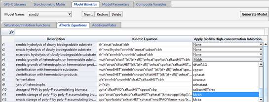
Figure 14‑17 - Applying Biofilm High Concentration Inhibition
Entering Model Variables and Parameters
On the “Model Parameters” page, enter all of the model stoichiometry in the “Stoichiometric Parameters” tab. Right-click on a row to add new parameters, if required.
Next, click over to the “Kinetic Parameters” tab, and enter the parameters of the model and their values and units. If the parameter is temperature sensitive, you can list values for 10C and 20C, or Arrhenius coefficient. Right-click on a row to add new rows if required.
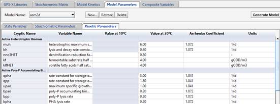
Figure 14‑18 - Defining the Kinetic Parameters in the ASM2d Model
Generating Models
Once the matrix and all other tabs have been filled out, the model can be generated. Note that the model will be generated for the library showing in the Library: pull-down menu on the GPS-X Libraries page.
The model is generated by pressing the “Generate Model” button, as shown below.
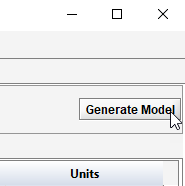
Figure 14‑19 - Generating a Model in Model Developer
You will be prompted to enter the full path to the GPS-X library where the new model will be written, as shown below:
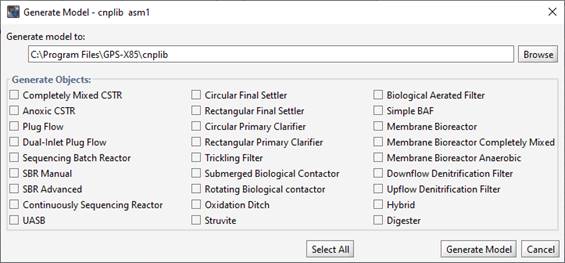
Figure 14‑20 - Generating a Model in Model Developer
Once you’ve entered the appropriate paths, you can select which unit processes should be generated (plug flow, MBR, etc.). Use the “Select All” button to generate models for all objects. MD will write out the files containing all the models. This may take up to a minute, depending on the speed of the computer.
Once the models have been written, close MD, and restart GPS-X. Select the library where the new models were written from the pull-down library menu at the top of the GPS-X screen.
When you select one of the objects selected in the Generate Model window (CSTR, plug flow tank, etc.), you will see the new model available under the Models menu.
A Note About Using Your New Models
Because your new model is not part of the original GPS-X structure, you will not be able to select it from the “Biological Models” menu in the influent object menu, and the Influent Advisor tool will not be available for your model. We recommend using the STATES influent model to simplify influent characterization when using custom biological models.
Technical Support and Troubleshooting
If you have any difficulties using Model Developer, or properly incorporating the models into GPS-X, please contact Hydromantis/Hatch.
References
Henze M, Grady C P L, Gujer W, Marais G v R and Matsuo T (1987). Activated sludge model no. 1. IAWPRC Scientific and Technical Report No. 1, IAWPRC, London.
Henze, M., W. Gujer, T. Mino, T. Matsuo, M.C. Wentzel, G.v.R. Marais and M.C.M. van Loosdrecht. (1998). Outline - Activated sludge model no. 2d. Proceedings of the Specialized Conference on Modelling and Microbiology of Activated Sludge Processes, Kollekolle, Denmark, 16-18 March.