Tutorial 17
Problem Statement
The integration of Python in GPS-X allows you to customize how you use GPS-X and while there is a wealth of open-source libraries available for Python, there may not always be a library available that meets your needs. To offer additional functionality to Python in GPS-X, the ability to add Java JAR files has been included. This will allow you to easily access JAR files to offer additional tools to customize your GPS-X experience.
The GPS-X Advanced Tools module is required to complete this tutorial.
Objectives
The purpose of this tutorial is to develop an understanding of how Python can be used to access Java JAR files within GPS-X. In this tutorial, we will look at how JAR files can be added to GPS-X and then we will use these JAR files with the Java Virtual Machine to visualize the difference between a GPS-X simulation run with and without the steady state box checked.
Adding Jar Class Paths
To use Java with Python in GPS-X, you must first provide GPS-X with a pathway to the JAR files that you would like to use. In this tutorial we will be using JAR files from JFreeChart, an open-source Java framework that is used for generating a variety of interactive charts. These JAR Files have already been added to the JAR Classpath in GPS-X, but the following steps will outline the process required to add JAR files to the GPS-X JAR Classpath.
1. Open a blank GPS-X layout.
2. Open the Python Preferences. The Python preference menu can be opened by going View > Preferences on the main toolbar. Open the Python tab.
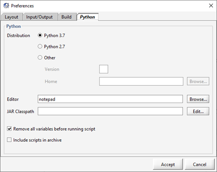
Figure 17‑1 - The Python Preferences Menu
3. Edit the JAR Classpath. Press the Edit… button next the JAR Classpath entry field to open the JAR Classpath Manager.
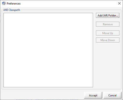
Figure 17‑2 - JAR Classpath Manager
4. Add the JAR Classpath. Press the Add JAR/Folder… button to open directory. Locate the JAR or folder of JARs you would like to add to the JAR Classpath. Press the Add JAR/Folder button to add it to the JAR Classpath.
5. Accept the JAR Classpath. Press the Accept button on the JAR Classpath Manager to return to the Python preferences manager.
6. Accept the new Python Settings. Press Accept on the Python preferences screen and you will be prompted to restart GPS-X for the new changes to take effect. Press OK to accept the changes to the Python preferences and close GPS-X.
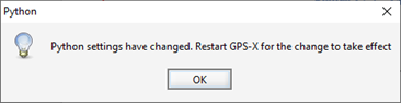
Figure 17‑3 - GPS-X Prompt to restart Python for the New Preferences to take Effect
Using JARS to Create Real Time Plots
7. Open GPS-X and open the layout created in Tutorial 1. Save the layout as ‘tutorial-17’.
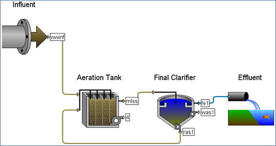
Figure 17‑4 - Layout used in Tutorial 17
8. Make the following changes to the layout:
· Change the Influent Flow Type, which can be found under Influent > Flow > Flow Data > Flow Type to Sinusoidal
· Change the Influent Flow Rate which can be found under Influent > Flow > Flow Data, to 3,000 m3/day
9. Switch to Simulation Mode.
10. Save the Layout.
11. A Python script has already been created for use in this tutorial. Locate and open the Python script called ‘tutorial-17.py’. The Python script can be found in the following directory:
\layouts\08tutorials\
12. Save the Python Script. Save the script in the current working directory.
13. Add the Script to GPS-X. Open the Python Script Manager in GPS-X and add the Python script to GPS-X.
14. Edit the Script. Press the Edit button to open the script in Notepad. This script is broken into two primary sections Functions and Plotting. We will now explore what the script is doing:
The Function section contains the standard GPS-X functions included in the GPS-X new Python script template. The cint() function is used to collect data at every communication interval. An additional user defined function, createDialPlot, has also been added to this section. This function is used to create and format a Dial plot in the Java Virtual Machine.
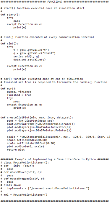
Figure 17‑5 - Functions Section of the Non-Steady State Test Python Script
The Plotting section of the script runs the simulation and creates a JPanel that a Dial plot and an XY line chart will be added to. The Dial Plot is used to track the time that has been elapsed in the simulation while the XY Line Chart visualizes the changes in xras1, the solids concentration in the secondary clarifier recycle stream.
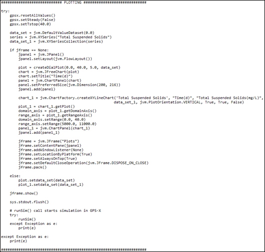
Figure 17‑6 - Plotting Section of the Non-Steady State Test Python Script
Two new GPS-X recognized Python commands are introduced in this section:
· gpsx.resetAllValues. This command is used to reset the value of all variables in the GPS-X layout back to their value default value defined when the active scenario was initially defined. No input is required for this command.
· gpsx.setSteady. This function allows you to toggle the GPS-X steady state status with Python. To check the set steady state box, type True in the parenthesis. To uncheck the steady state box, type False in the parenthesis.
15. Save the Script.
16. Run the Script. Press the Run Script button with the script highlighted to run the 40-day simulation with the steady state box unchecked.
17. By viewing the plot produced at the end of the simulation, as seen in Figure 17‑7, it can be noted that the total suspended solids in the secondary clarifiers recycle stream is initially very high and unpredictable. As the simulation continues to run, the level of total suspended solids reflects the sinusoidal influent pattern. After approximately 30 days, the output exhibits a constant upper and lower limit of total suspended solids in the recycle stream as a function of the influent flow. This plot is a visual representation of a plant reaching steady state operation. Minimize the Plots window so it is available to compare to the results of our next simulation.
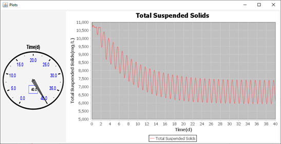
Figure 17‑7 – Non-Steady-State Python Script Output
18. Update the Python Script. We will now update the script so that it starts the simulation at steady state. Change the value fed to the gpsx.setSteady to True. Additionally, change the y-axis limits on the chart, defined by the rangeAxis.setRange(5000.0, 11000.0) command, such that the upper limit is 8,000 mg/L of total suspended solids.
19. Save the Python script.
20. Run the Python Script. Open the Python Script Manager. Run the script by pressing the Run Script button.
The results of the script can be seen in Figure 17‑8. The total suspended solids in the secondary clarifier recycle stream exhibits a sinusoidal pattern with constant maximum and minimum bounds.
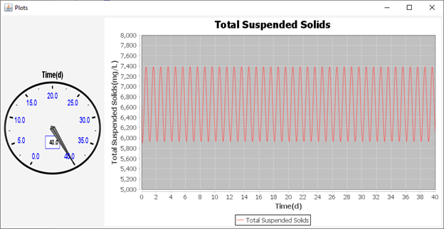
Figure 17‑8 - Steady State Test Python Script Output
21. If Figure 17‑8 is compared to the plot shown in Figure 17‑7, it can be observed that the simulations with and without the steady state box checked converges to the same results by the end of the simulation. These figures allow us to visualize the functionality of the steady state box in GPS-X. Checking the box finds a set of conditions that represent operating the plant at the input parameter settings defined in the GPS-X layout for a long period of time without disturbance. The simulation is then started from these conditions allowing you to simulate how disturbances would impact the plant operating at these steady state conditions. With the steady state box unchecked, the simulation begins from the initial conditions specified in the GPS-X definition. When starting from these conditions, it took the plant nearly 30 days to reach steady state operating conditions, despite operating under constant operating conditions without disturbance