Tutorial 16
Problem Statement
When creating a new model, it is common to preform a sensitivity analysis to analyze the effects that uncertainty in your parameters will have on the model. While visualizing the effects of changing a single parameter may offer the user a way to test the validity of a given model, it is often difficult to visualize the effects that simultaneously changing multiple parameters will have on the model.
By systematically altering the parameters used in a given system, you can develop a detailed understanding of how the variables in your model interact with each other. Through the use of Python, the analysis process in GPS-X can be simplified and you can create detailed sensitivity maps to visualize the relationship between variables in your system.
In this tutorial, the sensitivity of a plant’s effluent ammonia will be examined using two different methods. First, we will look at the sensitivity of effluent ammonia to simultaneous changes to both liquid temperature and the secondary clarifier’s wastage flow rate by producing a 3-Dimensional sensitivity map. We will then explore how various sets of operating conditions can be compared to each other directly on a 2-Dimensional plot using scenarios in GPS-X.
The GPS-X Advanced Tools module is required to complete this tutorial.
Objectives
The purpose of this tutorial is to see how Python can be used to maximize the information you extract from GPS-X. By the end of this tutorial, you can use Python to create detailed sensitivity analysis in GPS-X.
Plots in this section will be created using the matplotlib library in Python which must first be installed into Python, as described in Tutorial 14. The Python Pillow library (commonly referred to as PIL), will be used to open and display figures saved to files in this tutorial. If you would like to use Pillow library to open figure files after script execution, please install this library using the appropriate instillation command described in Tutorial 14. Otherwise, figure files will be saved in the same directory as the layout.
Two Manipulated Variable Sensitivity Analysis
We will now look at how Python can be used to model the sensitivity of an output variable to two simultaneously manipulated inputs. Ensure matplotlib and Pillow have been installed to the instance of Python you are using as described in Tutorial 14 before proceeding with this Tutorial.
1. Open the layout created in Tutorial 1 and save it as ‘tutorial-16’.
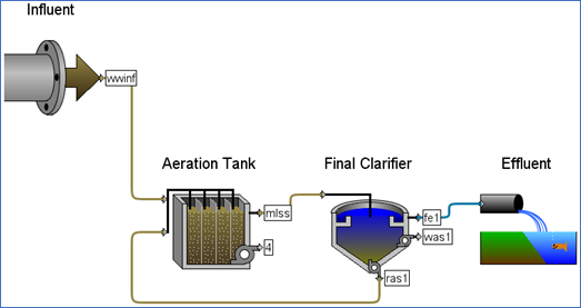
Figure 16‑1 - Tutorial 16 Layout
2. Switch to Modelling Mode if not already there.
3. Right click on the Influent object and select Composition > Influent Characterization to open the influent advisor.
4. Press the Raw button found in the toolbar at the bottom of the Influent Advisor tool window. This will revert any changes in the influent advisor to the default settings for a raw plant influent.
![]()
Figure 16‑2 - Influent Advisor Toolbar
5. Right click on the Secondary Clarifier and select Input Parameters > Operational.
6. Change the pumped flow variable back to the default setting of 40 m3/d. Note that hovering the mouse cursor over a modified variable will show you the GPS-X default value for that variable. Press Accept.
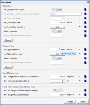
Figure 16‑3 - Displaying Default Variable Settings
Click on the Site Properties Button and navigate to the Plant Wide Properties Tab. Change the liquid Temperature back to the default value of 20 degrees Celsius.
7. Click on the Site Properties button and navigate to the Plant Wide Properties tab.
8. Change the Liquid Temperature value back to the default of 20°C. Press Accept.
9. Switch to Simulation Mode.
10. Open the Existing Python Script. We have included a Python script that has already been written to perform the sensitivity analysis. Locate and open the ‘tutorial-16-3D.py’Python script found in the following subdirectory of the GPS-X installation:
\layouts\08tutorials\
11. Save the Python Script. Save the script in the current working directory.
12. Open the Python Script Manager. The Python Script Manager can be accessed by through Tools > Python Script Manager on the main toolbar.
13. Add the Script to the Python Script Manager. Press the Add button and select tutorial-16-3D.py from the menu. Press Open to add it to the Python Script Manager.
14. Edit the Script. Press the Edit button to open the Python script in Notepad.
The script is broken into 4 major sections:
· User Inputs:
The user inputs section is where the user can define the range of values they would like to include in the sensitivity analysis. The user can specify upper and lower bounds for both the liquid temperature and the Secondary Clarifier wastage flowrate.
The user can also specify the number of points they would like to use in the sensitivity analysis. The range between the minimum and maximum values assigned to each variable will be split into this many equally spaced points. A simulation will be run at each of these conditions.
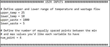
Figure 16‑4 - The User Inputs Section of the Python Script
· Functions:
The functions defined by GPS-X when creating a new Python script are used to manipulate variable values in GPS-X. In the start function, the values of temperature and wastage rate in GPS-X are being assigned the value of the current_temp and current_waste Python variables respectively. In the eor function, the effluent ammonia is assigned to the global variable current_ammonia, to be used in the Python script outside of the GPS-X simulation.
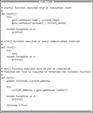
Figure 16‑5 - The Function Section of the Python Script
· Data Collection:
This section of the script creates the range of values to be looked at using Python’s numpy library. Using numpy, a coordinate matrix is constructed for each of the variables. The values in the matrices are equally spaced between the minimum and maximum values defined in the user inputs section. Each possible combination of these coordinates is then feed into the GPS-X simulation using global variables to determine the effluent Ammonia concentration under these operating conditions. These effluent concentrations are extracted from GPS-X and recorded in a results matrix.
A new GPS-X recognized function is also being used in the data collection code block gpsx.resetSim(). This function resets the GPS-X model, like pressing the Reset Model button in the GPS-X interface.
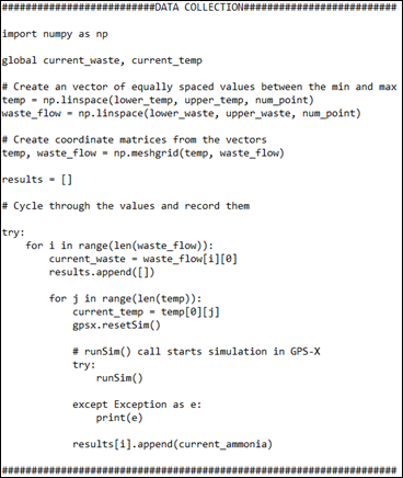
Figure 16‑6 - The Data Collection Section of the Python Script
· Plotting:
This section uses Python’s matplotlib library to create a 3-D plot of the data collected in the previous section of the Python script. The plot will be saved as a .png file in the same directory as the layout file at the end of the Python Script. Pillow is then used to open this PNG file prior to terminating the script.
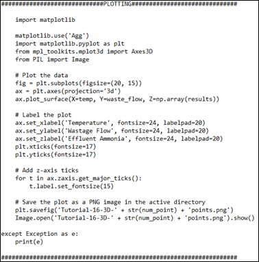
Figure 16‑7 - The Plotting Section of the Python Script
15. Save the Python Script.
16. Run the Python Script. Press the Run Script button on the Python Script Manager window.
17. View the Results. The plot will automatically be opened at the end of the script if you have installed the Pillow Python library. If you have not installed this library, the plot produced by the script is saved as a .png file in the directory where the layout file is saved. Open the directory where you have saved the layout file and locate the PNG file named “Tutorial-16-3D-4points.png”. Open the PNG file to view the results of the sensitivity analysis. Please ensure that Pillow library is installed to have Python automatically open the file at the end of executing the script.
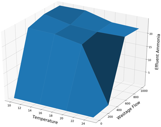
Figure 16‑8 - Sensitivity of Effluent Ammonia to Liquid Temperature and Wastage Flow
18. Edit the Python Script. In the User Inputs section of the Python script, make the following change:
· Increase the NumPoint value to 10 (This will increase the resolution of the of the data as more points are being sampled allowing you to better visualize trends). Note: The increased number of points will require more simulations and will take longer to run than the previous script.
19. Save the Python Script.
20. Run the Python Script.
21. View the Results. The new PNG figure found in the active directory called “Tutorial-16-3D-10points.png”. Notice that the resolution of the plot has increased due to the increased number of sample points being used.
Note: When deciding on the number of points to use in a sensitivity analysis, keep in mind that the number of simulations required does not grow linearly with the number of points. A large number of points to be examined can lead to long wait times depending on the speed of your machine and the complexity of your layout.
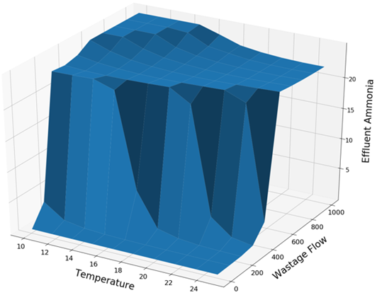
Figure 16‑9 - Sensitivity of Effluent Ammonia to Liquid Temperature and Wastage Flow with an Increased Number of Sample Points
Multi-Variable Sensitivity Analysis
We will now examine how we can visualize the effects of changing multiple variables in a simulation at once by using both GPS-X’s Scenario functionality and the matplotlib Python Library
22. Create Two New Scenarios. Information on creating new scenarios can be found in Tutorial 3. Create the two new scenarios with the following specifications:
· High Flow:
oDerived new scenario from: Base Model
oChange Influent Flow Rate, found under Influent > Flow > Flow Data, to 4,000 m3/day
oChange Aerator maximum volume, found under Aeration Tank > Input Parameters > Physical, to 1,500 m3
· Low Flow:
oDerived new scenario from: Base Model
oChange Influent Flow Rate, found under Influent > Flow >Flow Data, to 500 m3/day
oChange Aerator volume, found under Aeration Tank > Input Parameters > Physical, to 750 m3
23. Open the Existing Python Script. We have included a pre-written Python script that will perform a 2-Dimensional sensitivity analysis. Locate and open the tutorial-16-2D.py Python script found in the following subdirectory of the GPS-X installation directory:
\layouts\08tutorials\
24. Save the Python Script. Save the script in the current working directory.
25. Open the Python Script Manager.
26. Add the Script to the Python Script Manager. Press the Add button and select tutorial-16-2D.py from the menu.
27. Edit the Script. Press the Edit button to open the Python script in Notepad. The script is setup using the same 4 sections as the previous script. We will now walkthrough what each section does:
· User Inputs:
The user must define the temperature range they are interested in viewing and the number of equally spaced points they would like this range to be broken into. You can also specify the target effluent ammonia concentration, which will be superimposed on our output graph.
0-day simulations with a constant wastage flow will be conducted in the simulation. The value of these variables is set at the end of the user inputs section.
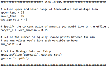
Figure 16‑10 - The User Input Section of the Python Script
· Functions:
The functions defined by GPS-X when creating a new Python script are used to manipulate to collect the concentration of ammonia leaving the plant.
A user defined function, gpsxFn(), has also been defined in the Functions section of the script. The gpsxFn() function is used to manage the characteristics of the GPS-X simulations being executed. The gpsxFn() function sets the value of liquid temperature in GPS-X. Additionally, the gpsxFn() uses a new GPS-X recognized Python function, gpsx.setScenario, to set the active scenario in GPS-X. The GPS-X simulation will be executed using this scenario next time runSim() is called. Refer to Tutorial 3 for more information on GPS-X scenarios.
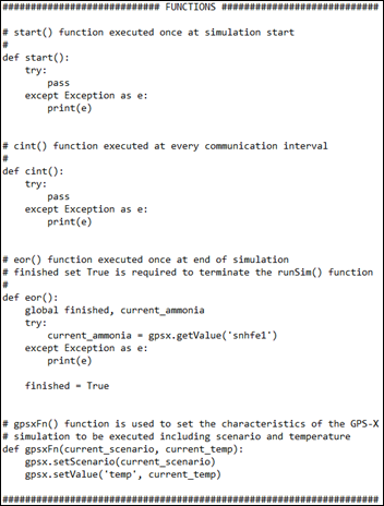
Figure 16‑11 - The Function Section of the Python Script
· Data Collection:
The temperature range to be examined is converted to a vector of equally spaced points in this section. This vector is then cycled through and each temperature in the vector is applied to each GPS-X scenario being analyzed. The effluent ammonia in each scenario is extracted from GPS-X and recorded to a scenario specific list of results in Python.
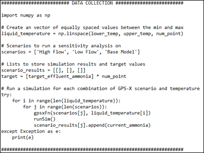
Figure 16‑12 - The Data Collection Section of the Python Script
· Plotting:
The results of the simulations are plotted on a single axis. A dashed line representing the target effluent ammonia concentration is plotted on the graph. The graph is then saved as a PNG file in the same directory the layout file is saved in with the name “Tutorial-16-2D-4points.png. Pillow will open this PNG at the end of the simulation.
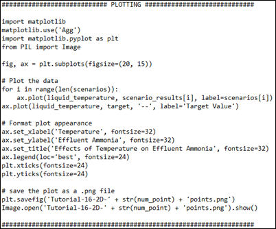
Figure 16‑13 - The Plotting Section of the Python Script
28. Save the Script.
29. Run the Python Script. Press the Run Script button on the Python Script Manager window.
30. View the Results. The plot produced by the script is saved as a .png file in the directory where the layout file is saved. Open the directory where you have saved the layout file and locate the file named “Tutorial-16-2D-4points.png”. Open the image file to view the results of the script.
From the results, we can see how the three different scenarios compare to each other. The Low Flow and Base Model scenarios are similar for all temperatures, but they both have a lower effluent ammonia concentration than the High Flow scenario at low temperatures. Using the superimposed target line, we can also determine that the Low Flow and Base Model scenarios have an acceptable effluent ammonia concentration at a liquid temperature of ~ 16.5 °C while the High Flow scenario has an acceptable effluent ammonia concentration at a liquid temperature of ~ 18.5 °C.
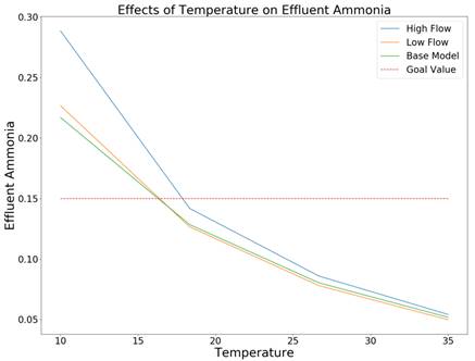
Figure 16‑14 - Effects of Liquid Temperature on Effluent Ammonia
31. Rerun the Script with new conditions. Increase the number of the number of points to be analyzed in the temperature range to 10. Increase the influent flow rate in the High Flow scenario to 5,000 m3/d.