Tutorial 15
Problem Statement
When building a model, it is often easy to overlook that many variables in the system may exhibit random behaviour. Additionally, if it is recognized that some variables, such as storm frequency and severity, historic data may be unavailable and creating data for the simulation may introduce an input bias to the system. By using Python, we can introduce truly unique data to the system and visualize how it will react.
By using random inputs, you can see how your wastewater treatment plant will react under unpredictable operating conditions. For example, when designing a plant, data may be available that details the influent that the plant can expect, but this data often omits random and unpredictable events such as storms that will impact your influent flow. Using Python’s random number generator, we will create a simulation to visualize the effects of storm frequency and severity on the influent flow rate to a plant and how this flow rate can be controlled.
The GPS-X Advanced Tools module is required to complete this tutorial.
Objectives
Upon completion of this tutorial, you will have an understanding of how Python’s random number generator can be used to generate random events in GPS-X and visualize the impact they have on the operation of your plant.
Setting Up the Layout
1. Create a new layout consisting of:
· A wastewater influent object,
· a stormwater runoff (Influent tab)
· a 2-flow combiner,
· a plug-flow tank,
· a circular secondary clarifier
· a wastewater outfall
Use the mantis2lib library and the default model selections (the codstatesinfluent model, the mantis2 plug flow tank model and the simple1d circular clarifier model).
Connect the unit processes and add the labels displayed in Figure 15‑1.
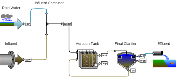
Figure 15‑1 - Tutorial 15 Layout
2. Save the layout as ‘tutorial-15’.
3. Enter Simulation Mode.
4. Create an output plot for the flow leaving the Influent Combiner as described in Tutorial 2 (Right click the 2-flow combiner object Output Variables > Flow). Name the plot “Total Plant Influent”, and set the plot to autoscale.
Creating a Random Event
5. Open the Existing Python Script. We have included a pre-written Python script for creating a random event. Locate and open the tutorial-15-Random.py Python script in the following subdirectory of the GPS-X installation:
\layouts\08tutorials\
6. Save the Python Script. Save the Python script in the same directory as the layout file.
7. Add the Python Script to the Layout. In the Python Script Manager press the Add button and select the script. Press Open.
8. Edit the Python Script. Press the Edit button to open the script in Notepad. The script has been broken into 2 sections:
· User Inputs:
The User Inputs section currently contains a list variable that corresponds to the rain fall depths that the Stormwater Runoff object can generate in mm/hr. It also contains a variable that will represent the user defined communication interval and stop time.
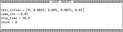
Figure 15‑2 - The User Inputs Section of the Python Script
· Functions:
The Functions section of the script contains the four functions that are automatically generated by GPS-X when creating a new Python script. Before the Start function, a new pre-defined GPS-X recognized command, gpsx.setCint is introduced. This command allows you to change the communication interval used in the GPS-X simulation directly within Python. To use the gpsx.setCint command, enter the desired communication interval in the parenthesis.
The randomness in this script is introduced in the cint function. Python’s random library is imported in the start function and in the cint function, Python’s random library is used to generate random integer numbers. Using conditional formatting, these random integers are then used to assign a value to the rainfall depths variable in the Stormwater Runoff object, creating random behaviour in the simulation.
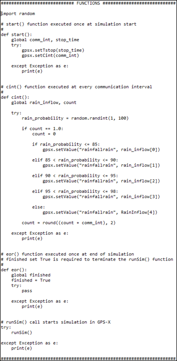
Figure 15‑3 - The Functions Section of the Python Script
9. Save the Python Script.
10. Run the Script. Press the Run button in the Python Script Manager. A sample output graph can be seen in Figure 15‑4. Note: Your graph will appear different than what is seen here due to the randomness introduced by the Python script.
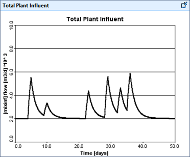
Figure 15‑4 - Output Graph of the Random Rain Event
Limiting Maximum Influent
With the introduction of a random rainfall event, the total influent to the plant may reach values that exceed the maximum capacity of the treatment equipment. To accommodate this, we will use Python to simulate a bypass weir.
11. Enter Modelling Mode.
12. Add the following objects:
· A Control Splitter (This will act as our bypass weir),
· a 2-flow Combiner
Adjust the unit connections and stream labels as seen in Figure 15‑5.
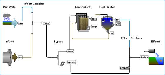
Figure 15‑5 - Tutorial 15 Layout with a Bypass Introduced
13. Switch to Simulation Mode
14. Add the following variables to the output plot created in Step 4:
o Total Influent Flow can be found in the Influent Combiner Output Variables > Flow
o The Aerator flow can be found by right clicking the wwinf connection point on the Control Splitter Output Variables > Flow
o The Bypass flow can be found by right clicking the bypass connection point on the Control Splitter Output Variables > Flow
o Rename the plot “Influent Bypass Operation, and set the plot to autoscale
15. Open the Python Script Manager
16. Edit the Python Script. Select the “tutorial-15-Random.py” Python script and hit the Edit button on the Python Script Manager.
17. Save the Script. We will be modifying the “tutorial-15-Random.py” Python script in our new scenario. To avoid changing the script used in the previous section, go to File > Save As. In the Save As window change the Save as type to All Files and save the script with a new name ending in .py extension (eg. “tutorial-15-Bypass.py”)
18. We will need to make the following changes to the Python script:
o Add the following to the User Input Section:
max_aerator_flow = 4000
This value represents the maximum allowable flow rate that the Aerator can handle.
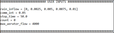
Figure 15‑6 - Changes to the User Inputs Section in the Bypass Python Script
o Add the following to the global variables defined at the start of the cint section:
max_aerator_flow
o Add the following to the end of the cint function:
inflow = gpsx.getValue('qmixinf')
if inflow > max_aerator_flow:
gpsx.setValue('qconbypass', (inflow – max_aerator_flow))
else:
gpsx.setValue('qconbypass', 0.0)
o These changes can be seen inside the red boxes in Figure 15-7
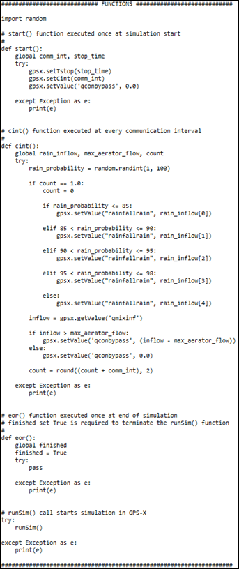
Figure 15‑7 - Changes to the Functions Section in the Bypass Python Script
This block finds the total influent that is entering the plant from both influent objects and determines if it is greater than what the Aerator can handle. If the influent flow rate is greater than the maximum aerator flow rate, the excess is bypassed.
19. Save the Script.
20. Add the Python Script to the Layout. In the Python Script Manager press the Add button and select the script. Press Open.
21. Run the Script. A sample output can be seen in Figure 15‑8. Note: your output will appear different due to the randomness in this script.
Notice that by controlling the bypass this way, any flow that would exceed the maximum allowable aerator influent of 4,000 m3/d is instantaneously bypassed and the influent limit is never exceeded.
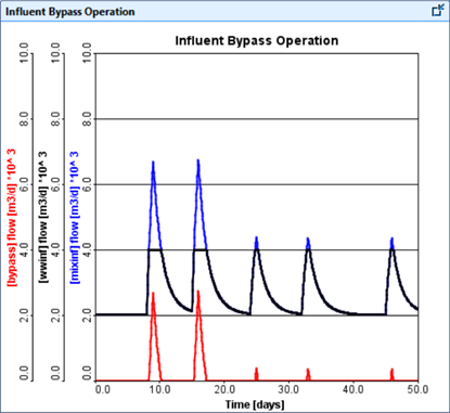
Figure 15‑8 - Output of the "tutorial-15-Bypass" Python Script
Creating an Input Delay
When running a GPS-X simulation, changes caused by control loops happen instantaneously, but this assumption does not always translate directly to the real world as input delays and equipment start up times may cause a discrepancy between the detection of an event and when it is corrected for. We will now look at how we can use Python to delay the time it takes for the model to address a deviation from setpoint.
22. Open the Existing Python Script. We have included a Python script that has already been written to delay the bypasses’ ability to control the influent. Locate and open the tutorial-15-Delay.py Python script in the following subdirectory of the GPS-X installation directory:
\layouts\08tutorials\
23. Save the Python Script in the active directory
24. Open the Python Script Manger
25. Add the Script to the Python Script Manager
26. Edit the Script. This Python script is built from the “tutorial-15-Bypass.py” Python script. We will now discuss the changes made from that Python script:
27. influent: A list variable called influent has been added to the start function. This variable is used in the cint function to collect the total influent flow at every communication interval.
28. count: A variable called count has been added to the start function. This variable is used to track the number of communication intervals that have occurred. The communication interval time has been reduced in this Python script, so the count variable tracks the communication intervals to ensure the random event still occurs on the communication interval that corresponds to 1 day being elapsed.
29. Bypass Control: The bypass control from the previous Python script has been modified and now compares the total influent flow that occurred 5 confidence intervals prior to the maximum allowable flow rate to the aerator. This introduces a delay of 5 communication intervals to the bypasses ability to control a deviation in the influent flow rate.
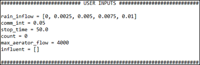
Figure 15‑9 - Changes to the User Inputs Section of the Delayed Bypass Python Script
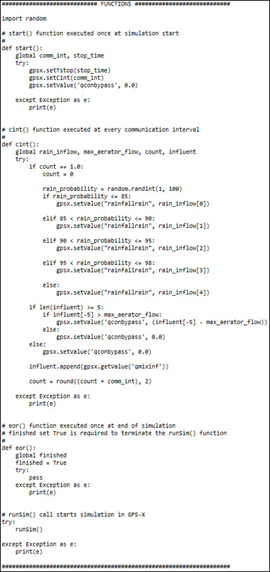
Figure 15‑10 - Changes to the Functions Section of the Delayed Bypass Python Script
30. Save the Script
31. Run the Script. A sample output can be seen in Figure 15‑11. Note: your output will appear different due to the randomness in this script.
Notice that when the Aerator influent limit is exceeded, the bypass does not immediately activate, and excess influent enters the Aerator. It can also be noted that when the bypass is activated, that the amount bypassed exceeds what is actually required to meet the maximum influent allowed to enter the aerator.
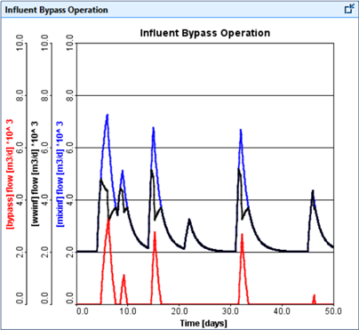
Figure 15‑11 - Output of the "tutorial-15-Delay" Python Script