Tutorial 13
Problem Statement
When developing a plant model, we may wish to not only explore what loads a plant will fail under, but the frequency with which these failures might occur. While linear analysis can tell us at which points the plant will fail, Monte Carlo analysis allows us to determine the frequency with which the plant will fail.
Monte Carlo analysis is also useful in exploring plant performance under different design assumptions. For example, when designing a plant, you need to choose a value for the autotrophic maximum specific growth rate and the alpha factors for your reactors. Neither of these values can be fully known in advance, however we can approximate the range in which these values will fall. We may know that the alpha factor for the waste water will fall somewhere between 0.4 and 0.7 and that the probability of it being any particular number inside this range is uniform. By assigning probabilities to the range of values we can use Monte Carlo analyses to not only investigate the plant’s performance over the range but the probability of the observed performance characteristics.
Objectives
The purpose of this tutorial is to develop a basic understanding of Monte Carlo analysis in GPS-X. Upon completion of this tutorial you will be able to carry out Monte Carlo analysis of model variables. In this tutorial, we will be looking into how the dissolved oxygen in the tank reactor and free and ionized ammonia in the plant effluent are affected by various alpha factors and autotrophic maximum specific growth rates.
The GPS-X Advanced Tools module is required to complete this tutorial.
Setting Up the Layout
The Analyze module is an optional feature of GPS-X. If you have not purchased this module, contact us for pricing information.
1. Because this feature requires multiple simulations, for demonstration purposes the work will be carried out on a simple model consisting of a Wastewater Influent, a Completely-Mixed Tank, and a Rectangular Secondary Clarifier. Start a new layout.
2. Select the Comprehensive (mantis2lib) from the Library menu (if it isn’t already selected) (see Figure 13‑1)
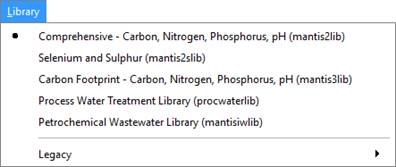
Figure 13‑1 - Select Library
3. Create the layout as shown in Figure 13‑2 with a codstates influent model, mantis2 CSTR model and simple1d clarifier model.
4. Save the layout with the name ‘tutorial-13’.
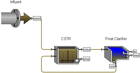
Figure 13‑2 - Tutorial 13 Layout
|
|
5. Simulate cold winter conditions. Access the Plant Wide Properties by pressing the button in the upper left corner of the drawing board. Change the liquid temperature to 10°C. |
6. Change CSTR parameters.
· Set Input Parameters > Operational > specify oxygen transfer by to Entering Airflow.
· Set the total air flow into aeration tank to 15,000 m3/d.
7. Change the clarifier parameters.
· Set Input Parameters > Operational > pumped flow to 70 m3/d.
8. Save the layout.
9. Switch to Simulation Mode.
10. Create input controls. From the CSTR object, drag the following parameter to a new input control tab:
· maximum growth rate for ammonia oxidizer from Input Parameters > Kinetic (Ammonia-Oxidizing Biomass section)
· maximum growth rate for nitrite oxidizer from Input Parameters > Kinetic (Nitrite-Oxidizing Biomass section)
· alpha factor (fine bubble) from Input Parameters > Operational. Under the Diffused Aeration section, click on the ‘More…’ button. Next to the alpha factor click on the ellipsis (…) button and add the ‘fine bubble’ variable to the input control tab by clicking and dragging from the numeric entry field.
11. Edit the controller settings. Open the properties window and change the maximum growth rate for ammonia oxidizer settings to:
· a min/max of 0.5 and 1.2, respectively.
· the controller type to “Analyze – Monte Carlo”. Notice that a button icon appeared beside the Type box. This allows you access to the Distribution settings.
· edit the Distribution settings and change the Type to Normal, the mean to 0.9, and the standard deviation to 0.1.
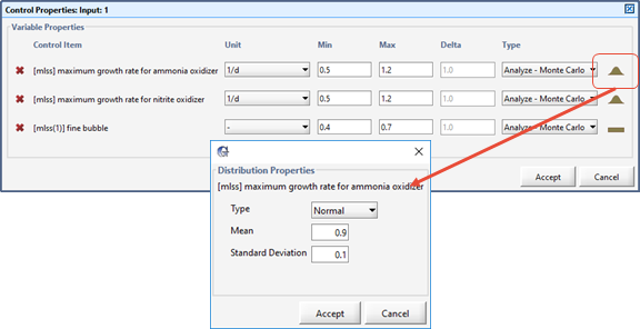
Figure 13‑3 – Monte Carlo Controller Settings
Similarly, for the maximum growth rate for nitrite oxidizer, change the min/max to 0.5 and 1.2 and change the type to “Analyze – Monte Carlo”. Also change the distribution to Normal but, in this case, change the mean to 1.0 and the standard deviation to 0.1.
This allows the two parameters to vary about the default model settings.
For the alpha factor, set the min/max to 0.4 and 0.7 and the controller type to “Analyze – Monte Carlo”. Leave the distribution as Uniform.
12. Create another input control. We will also want to vary the number of Monte Carlo runs, so we’ll create another input controller for the number of runs. That variable can be found from the main menu in:
Layout > General Data > System > Input Parameters > Simulation Tool Settings
We will now set up separate output graphs of our input (to see the input distributions that were generated) and output (which will tell us how well the plant performed).
13. Create graphs of our input variables. Note that these are the output variables representing the input parameters. You can’t drag the input parameter itself to a graph.
Create an output tab labeled “Input Distributions” and add the following parameters to their own separate graphs:
· maximum growth rate for ammonia oxidizer from the CSTR’s Output Variables > Input Parameters > Kinetic (Ammonia-Oxidizing Biomass header) menu.
· maximum growth rate for nitrite oxidizer from the CSTR’s Output Variables > Input Parameters > Kinetic (Nitrite-Oxidizing Biomass header) menu.
· aeration alpha from the CSTR’s Output Variables > Oxygen transfer. Under the Standard Oxygen Transfer Efficiency section.
14. Create graphs of our output variables.
Create an output tab labeled “Output Distribution” and add the following parameters to their own separate graphs (from the CSTR’s Output Variables > Concentrations form):
· dissolved oxygen,
· ammonia nitrogen,
· nitrite
· nitrate
15. Edit the graphs’ settings.
For all of the graphs on both tabs, change:
· the graph type to Probabilistic (Monte Carlo)
· select Autoscale for both the x and y axes
This graph type will plot a histogram of our Monte Carlo results.
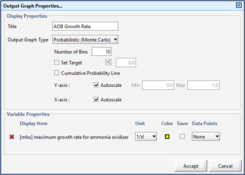
Figure 13‑4 – Monte Carlo Graph Properties
In addition, for the dissolved oxygen and ammonia nitrogen graphs, set:
· the number of bins to 20 (to see the distribution at a higher resolution)
· the target values to < 3.0 for ammonia nitrogen and >2.0 for dissolved oxygen (you can change the sign of the <, > symbol by left-clicking on the icon)
16. Save the layout.
Selecting Analyze Mode
|
|
17. Select the Monte Carlo analysis type. Click the little arrow beside the Analyze button on the main toolbar (or access it through the main menu’s Tools > Analyze) and select “Monte Carlo”. |
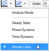
Figure 13‑5 - Selecting Analysis Type
Switch to Analyze Mode. Click the Analyze button on the main toolbar (or access the Analyze Mode checkbox through the main menu’s Tools > Analyze) to turn on the analyzer.
The status bar at the bottom right of the main window will indicate that you are in Analyze Mode.
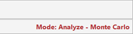
Figure 13‑6 - Status Bar showing “Analyze – Monte Carlo” Mode
Running Simulations
18. Run the simulation. The simulations will run one after another, while collecting the output of the model for post-simulation analysis. You can follow the progress of the simulations on the Input tab, as the red indicator on the three input parameters progresses through the required simulations (1000 of them, by default). Note that it may take several minutes for the simulations to complete, depending on the speed of your computer.
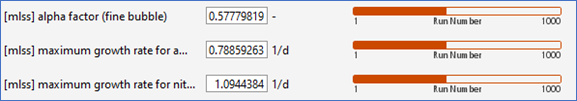
Figure 13‑7 - Tracking the Progression of the Simulations
When the simulations are completed you should see the distribution of input parameters for the alpha constant and the two growth rates. The growth rates should follow a normal distribution, whereas the alpha factor should have a uniform (flat) distribution. Note that the distribution of actual values used may not quite fit the expected distribution shape. This is due to only running 1000 simulations – it would be more representative of the desired distribution with larger numbers of simulations.
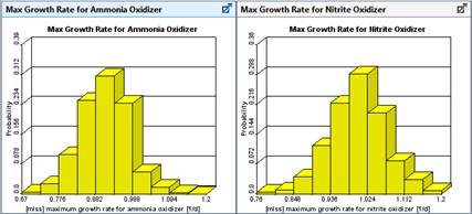
Figure 13‑8 – Input Parameter Distributions
The graphs on the Output Distributions tab shows the performance of the plant under the varying model input. The effluent ammonia graph illustrates that the plant is nitrifying most of the time. The target line shows that the plant effluent ammonia is equal to or less than the target 3.0 mgN/L in 88.6% of the simulations. Note that in the Monte Carlo analysis you may receive slightly different solutions but the % value recorded on the graph should be within the range of 85% to 90%.
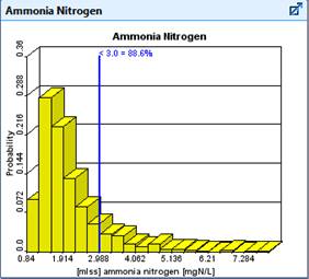
Figure 13‑9 – Output Distribution Results showing Target
19. Rerun the simulation. However, this time use a larger aeration capacity.Create a new scenario, and try increasing the aeration tank volume and/or the airflow to the system. How much larger does it have to be to have 95% of the simulations with effluent ammonia at 3.0 mgN/L or less?