Tutorial 12
Problem Statement
With many of the dynamic models used in GPS-X most of the model parameters are assumed to be constant over the entire calibration period. For example, the clarifier's flocculent zone settling parameter is normally set to one specific value for the entire simulation. One reason for doing so is that it is difficult to determine or identify the changes in this parameter over time since it is difficult to measure on-line. The best the modeler can do is assume that the parameter does not change over the simulation period, and therefore use only one value to fit the target or measured data.
A more rigorous approach, however, might be to try to fit the measured data by varying the parameter over the simulation period. This has two advantages: a better agreement between the model and data, and an indicator of the dynamic response of the parameter. Of course, this technique assumes that the measured data is relatively free of error.
Objectives
After completing this tutorial, you should be able to set up and run the dynamic parameter estimator (DPE). The GPS-X Advanced Tools module is required to complete this tutorial.
Setting Up the Layout
1. Load the starting point layout. We have already set up a layout with the appropriate data files, controllers, and output graphs. You can find it by going to File > Sample Layouts > Tutorials> Tutorial 12 – Dynamic Parameter Estimation (Starting Point).
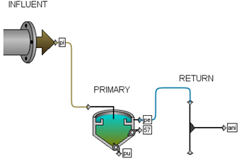
Figure 12‑1 - Layout used in Tutorial 12
2. Save the layout as a different name in your own directory. We are going to be making some changes and we would like to leave the starting point layout as is.
3. Switch to Simulation Mode if not already selected.
4. Run a 4-day dynamic simulation with the steady-state box checked.
The graph of the primary effluent TSS shows a reasonable fit with the real measured data but there is considerable room for improvement. These results are shown in Figure 12‑2.
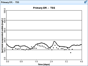
Figure 12‑2 – Primary Effluent TSS
Setting Up the DPE
At this point, it is desirable to improve the fit between the primary effluent TSS and the data by optimizing the flocculent zone settling parameter as it varies with time.
5. Switch to Modelling Mode.
|
|
6. Open the Optimize menu on the top toolbar and select Optimize Setup. This will display the Optimizer Setup Wizard. |
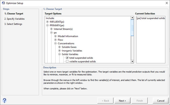
Figure 12‑3 - Optimize Setup Wizard (Target Variables)
7. Select the Target Variable. In this case, it is the total suspended solids in the reactor. It can be found under:
PRIMARY(pe) > pe > Concentrations > Solids Variables
8. Click Next to proceed to the next stage.
9. Select the Optimize Variable. In this case, it is the flocculant zone settling parameter in the reactor. It can be found under:
PRIMARY(pe) > Settling > Double Exponential Parameters
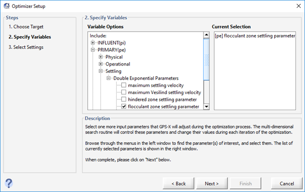
Figure 12‑4 - Optimize Setup Wizard (Optimize Variables)
10. Click Next to proceed to the next stage.
11. Specify Optimizer Settings. The last step in the process is to specify which kind of optimization we are doing. We will use Fit to Data, DPE, and Absolute Difference.
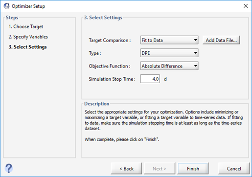
Figure 12‑5 - Optimize Setup Wizard (Optimizer Settings)
We can also use the “Add Data File…” button here to add data if needed, but we have already specified our data file, so we don’t need to do it again here.
12. Click Finish to complete the set up.
13. Switch to Simulation Mode.
Note that a new input panel has been created with our optimize variable already set to the optimize type. The target variable has also been plotted on a new graph.
14. Enter Optimization Mode. Open the Optimize menu on the top toolbar and select Optimize Mode.
15. Change the limits of the optimize variable. Edit the settings and change the min/max to 0.0001 and 0.005 respectively.
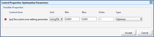
Figure 12‑6 – Optimize Parameter Limits
16. Save the layout.
17. Run the simulation. The results are shown in Figure 12‑7 and Figure 12‑8.
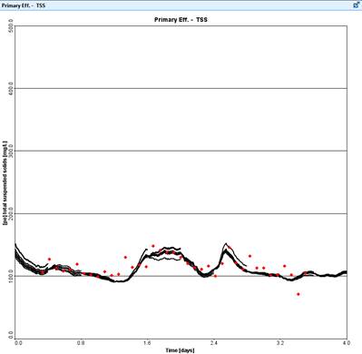
Figure 12‑7 – DPE Results
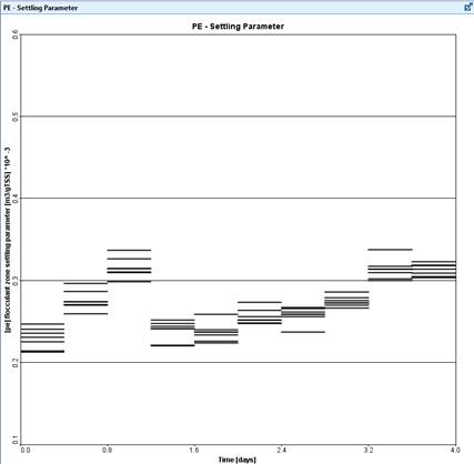
Figure 12‑8 – Flocculent Parameter
Try repeating the simulation with a shorter time window or tighter convergence criteria. These settings have been set up as input control sliders on the “DPE Settings” tab.