Tutorial 11
Problem Statement
No wastewater treatment plant modeling/simulation tool can be general enough to automatically handle ALL conceivable plant layouts or desired variables. So, GPS-X facilitates model layout customization. This is an advanced feature of GPS- X and requires a basic understanding of ACSL, the simulation language upon which GPS-X is based. The potential of the tool will be demonstrated using the following simple example.
In this tutorial, you will add two equations to calculate the specific oxygen uptake rate (SOUR) for the first stage of a plug-flow tank. One of the equations will assume an ideal oxygen uptake rate (OUR) measurement and the second will simulate measurement noise on the oxygen uptake rate measurement. This variable is often used for toxicity detection and in process control strategies.
Objectives
This tutorial is
designed to introduce you to the steps required to input your own
code for a specific plant layout. You will learn how to set
up the GPS-X interface, allowing you to input and output these
customized variables as if they were part of the original
layout.
Setting Up the Layout
1. Openthe layout completed in Tutorial 1 and save it as `tutorial-11’
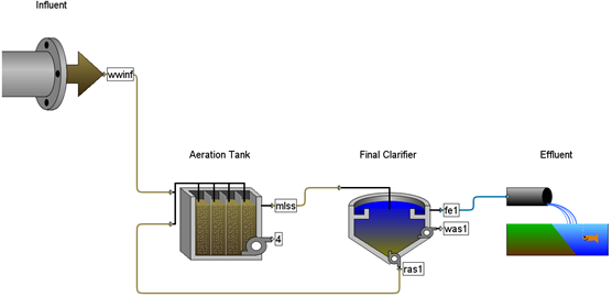
Figure 11‑1 – Tutorial 11 Layout
2. Switch to Modelling Mode.
3. Change the influent’s parameters.
· Set Flow > Flow Data > flow type to Sinusoidal.
4. Change the Aeration tank’s parameters.
· Set Input Parameters > Operational > specify oxygen transfer by… to Entering Airflow.
· Set the total air flow into aeration tank to 30,000 m3/d.
5. Save the layout.
7. Create a new graph. You will add the flow and a variable from the first reactor of the plug flow tank to the same graph.
· add flow from the influent’s Output Variables > Flow form
· add actual oxygen uptake rate from the first reactor. This is accessed through Output Variables > Internal Variables. Click the ellipsis button beside the variable to access the individual elements and drag the first element to the graph.
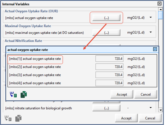
Figure 11‑2 – Accessing Individual Reactor Variables
8. Set the graph properties. In the Output Graph Properties window, set:
· the flow limits to 0-12,500 m3/d
· the OUR limits to 250-1,500 mgO2/L/d
Note: You may have to ‘unlock’ the min/max fields to edit them separately.
9. Save the layout.
10. Run a 10-day dynamic simulation (with the steady-state box checked) to ensure that the model is correctly set up. You should be able to produce a graph similar to Figure 11‑3.
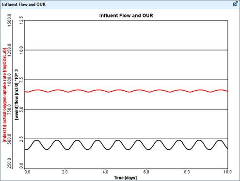
Figure 11‑3 – Example Graph from Dynamic Simulation
11. Switch to Modelling Mode.
Adding Custom Macros
12. Open the macros user file. This is done by choosing Layout > General Data > User Files > Macros from the main menu.
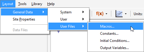
Figure 11‑4 - Accessing the Macro User File
In this file, which is generated when you save the layout for the first time, there are several sections separated by asterisks. They correspond to the different sections of the ACSL program structure. In this example, you will add new code to the DERIVATIVE SECTION as shown below.
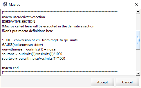
Figure 11‑5 – Adding Code to Derivative Section
13. Add the following code to the DERIVATIVE SECTION:
!1000 = conversion of VSS from mg/L to g/L units
GAUSS(noise=mean,stdev)
ourwithnoise = ourlmlss(1) + noise
sourone = ourlmlss(1)/vsslmlss(1)*1000
sourtwo = ourwithnoise/vsslmlss(1)*1000
The line starting with an exclamation mark is just a comment.
The other four lines create new variables (noise, ourwithnoise, sourone, sourtwo) and calculate values for them.
The variable noise makes use of an ACSL command, GAUSS to simulate measurement noise.
There are two existing variables used in the calculation (ourlmlss(1), vsslmlss(1)). These are the cryptic names of actual oxygen uptake rate and mixed liquor volatile suspended solids in reactor, respectively, from the first reactor in the plug flow tank. Remember that you can view these cryptic names by hovering over the variables label and viewing the tooltip (see Figure 11‑6).
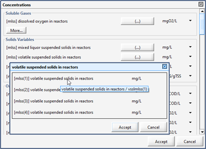
Figure 11‑6 – Viewing Cryptic Names
14. Click Accept in the Macros dialog to save the changes.
|
NOTE: This custom code is saved in a file called ‘tutorial-11.usr’ in the same directory as the layouts folder of your GPS-X V8.5 installation file directory. You can open and edit that file in an external text editor if you would prefer instead of using the GPS-X code editor. |
Adding Custom Input Variables
15. Add user-defined input variables. This is done by choosing Layout > General Data > User Files > Constants… from the main menu. This file allows you to set up the input variables on the same type of input forms as the other GPS-X variables.
16. Modify the code to read:
!MENU ITEM:!Noise Variables
!HEADER:!Noise Variables
constant mean = 0.0 !average measurement noise !gO2/(m3.d)
constant stdev = 50.0 !measurement noise standard deviation !gO2/(m3.d)
The MENU ITEM and HEADER lines set up the menus and groupings of the variables.
The lines that start with the keyword constant signify that this variable is an ACSL constant. This keyword is followed by the cryptic name, value, label and unit (with the appropriate delimiters shown above).
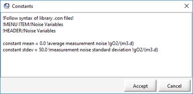
Figure 11‑7 – Adding User-Defined Inputs
17. Click Accept in the Constants dialog to save the changes. You will be prompted to reload your GPS-X layout.
|
NOTE: This custom code is saved in a file called ‘tutorial-11.con’ in the same directory as your layout. You can open and edit that file in an external text editor if you would prefer instead of using the GPS-X code editor. |
18. Save the layout and reload (close and reopen the file). This will cause GPS-X to read in your user-defined constants and create the menus associated with them. You will notice that there is now a menu item Layout > General Data > User > Input Parameters > Noise Variables.
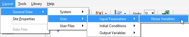
Figure 11‑8 - New User-Defined Input Parameters
Adding Custom Output Variables
19. Add user-defined output variables. This is done by choosing Layout > General Data > User Files > Output Variables from the main menu. This file allows you to set up the output variables on the same type of output forms as the other GPS-X variables.
20. Modify the code to read:
!MENU ITEM:!Uptake Variables
!HEADER:!Uptake Variables
display ourwithnoise !OUR with noise !gO2/(m3.d)
display sourone !SOUR without noise !mgO2/(gVSS.d)
display sourtwo !SOUR with noise !mgO2/(gVSS.d)
!MENU ITEM: !Noise Variables
!HEADER: !Noise Variables
display noise !measurement noise !gO2/(m3.d)
display mean !average measurement noise !gO2/(m3.d)
display stdev !measurement noise standard deviation !gO2/(m3.d)
The difference between the input variable file and this output variable file is that the keyword is ‘display’ instead of ‘constant’ and a value is not given for the output variables (because it will be calculated by the model).
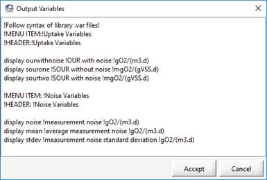
Figure 11‑9 – Adding User-Defined Outputs
21. Click Accept in the Outputs dialog to save the changes. You will be prompted to reload your GPS-X layout.
|
NOTE: This custom code is saved in a file called ‘tutorial-11.var’ in the same directory as your layout. You can open and edit that file in an external text editor if you would prefer instead of using the GPS-X code editor. |
22. Save the layout and reload. This will cause GPS-X to read in your user-defined constants and create the menus associated with them. You will notice that there are now two new menu items under Layout > General Data > User > Output Variables as displayed in Figure 11‑10.
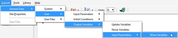
Figure 11‑10 – New User-Defined Output Parameters
Setting Up Simulations with Custom Variables
23. Switch to Simulation Mode.
24. Create input controllers. Place the 2 new input variables on sliders on the controls tab. These variables can be found in Layout > General Data > User > Input Parameters > Noise Variables.
25. Change the controllers’ settings.
· For the average measurement noise, set the limits from 0 to 100.
· For the measurement noise standard deviation, set the limits from 0 to 100.
26. Create a new graph. Place the 2 new SOUR variables (SOUR without noise and Sour with noise) on a graph. These variables can be found in Layout > General Data > User > Output Variables > Uptake Variables. Set the limits from 0 to 1200.
27. Add variable to existing graph. Place the OUR with noise variable on the existing graph that we created earlier in this tutorial (i.e. with flow and actual OUR). Set the limits from 250 to 1,500.
Running Simulations
28. Auto arrange the graphs and run a 10-day dynamic simulation with the steady-state box checked. You should produce a graph similar to Figure 11‑11.
29. Vary the noise parameters with the Input Control windows and observe the impact on the output. Try running several simulations using different settings.
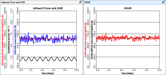
Figure 11‑11 – Simulation Results with Noise