CHAPTER 1
Starting GPS-X
|
Start GPS-X by either double-clicking on the GPS-X 8.5 icon on the desktop, or by accessing the “Hydromantis GPS-X 8.5” program group in the Windows “Start Menu”, and selecting “GPS-X 8.5” |
|

Elements of The Main Window
The basic elements of the GPS-X window are:
· Title bar
· Menu bar
· Toolbar
· Drawing Board
· Simulation Toolbar (in Simulation Mode only)
· Modelling/Simulation toggle button
A short description of each of these elements is provided below.
Title Bar
In addition to the buttons that control the appearance of the main window; the title bar area contains information about the version of GPS-X, the current layout being edited, and the library that this layout is using.
GPS-X 8.5 [<layoutname>] - <library>
Menu Bar
Most of the features of GPS-X are accessed from one of these six menus.
· File
· Edit
· View
· Layout
· Tools
· Library
· Help
Figure 1‑1 –Menu Bar
A brief description of each menu and their associated item(s) is provided below.
File Menu
The File menu contains items for performing file handling and manipulation.
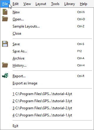
Figure 1‑2 - File Menu
New
Create a new session with a blank drawing board.
Open…
Opens a file browser where you can browse to and select an existing GPS-X layout file.
A preview pane is on the right which shows you the drawing board image of the selected layout file.
The Files of Type drop down box can be used to show only GPS-X layout files (.lyt extension) or only GPS-X archived layouts (.zip extension).
Sample Layouts…
Allows you to select from the 50+ pre-configured layouts that come with a licensed version of GPS-X.
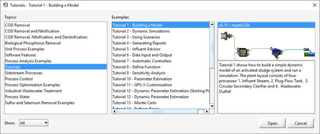
Figure 1‑3 – Sample Layouts Dialog
Close
Closes the current layout. If any changes have been made, you are prompted about saving or discarding the changes.
Save
Saves the current layout to a file. This command will overwrite the existing layout file having the same name (shown in the title bar) with the current layout information.
Save As…
This opens a file browser, which allows you to enter a layout file name and location before saving. The current layout information is saved to the specified file.
Archive
Creates an archive file (i.e. zip compatible file) of all the GPS-X files pertaining to the layout currently open. This is useful when transferring files between computers, or when sending files as attachments via email.
History…
A tool for managing multiple versions of a GPS-X layout. The option “Enable layout history” must be checked in the View > Preferences > Layout menu to allow access to the layout history management tools. Further details on the History menu can be found in CHAPTER 2 (Layout History Database)
Report…
Create a report with information about the current layout. See the Generating a Report section in CHAPTER 7 for more information.
Export as Image
Create a customizable image of the layout to export as a file. See the Exporting Layout Image section in CHAPTER 7 for more information.
Recent File List…
A list of recently opened layouts is shown at the bottom of the File menu. The number of layouts shown here can be set in the View > Preferences >Layout tab, under the Settings header.
Exit
Exits the program. You will be prompted to save or discard any unsaved changes to the layout.
Edit Menu
The Edit menu includes items related to manipulation of objects on the drawing board.
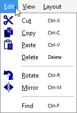
Figure 1‑4 - Edit Menu
Cut
Cuts the currently selected process(es) from the drawing board and places it on the clipboard.
Copy
Copies the currently selected process(es) from the drawing board and places it on the clipboard.
Paste
Pastes process(es) from the clipboard onto the drawing board.
Delete
Deletes the currently selected process(es) from the drawing board.
Rotate
Rotates the currently selected process(es) 90 degrees in the counterclockwise direction.
Mirror
Horizontally flips the currently selected process(es).
Find
The Find menu item brings up the “Find” dialog, which can be used to search for GPS-X variables by entering part of the plain text or cryptic variable name.
View Menu
The View menu button provides control over the look of the drawing board and how the object icons are displayed.
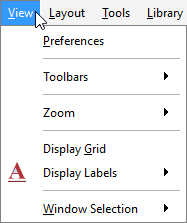
Figure 1‑5 – View Menu
Preferences
The Preferences menu item brings up the “Preferences” dialog, which contains a series of tabbed sheets including the Layout, Input/Output, Build, and Python tabs. This window is used to set the default preferences for new layouts including the default library at start up:
|
Layout |
details on default libraries, directories, etc., at startup, as well as settings for the look and feel of objects on the GPS-X drawing board. |
|
Input/Output |
default input controller and output graph types, plus details on report generation options. |
|
Build |
details on FORTRAN compiler and ACSL model build options. |
|
Python |
Details on the Python instance being used by GPS-X |
Toolbars → Process Table
Gives you the ability to hide/show the process table.
The process table consists of a collection of unit processes and control points that are used to build the model layout for a wastewater treatment plant. One or more copies of each object in this table can be dragged onto the drawing board.
The objects are arranged in groups of similar unit processes, such as Primary Treatment, Suspended Growth Processes, and Biosolids Treatment. Click on the group name to open the group and display the available objects.
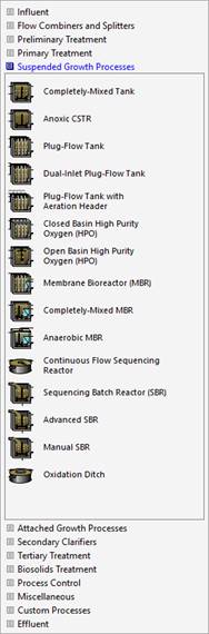
Figure 1‑6 – Process Table
Zoom
The Zoom menu item contains a series of options for adjusting the level of zoom applied to the drawing board. The total drawing board consists of a grid 32 blocks wide by 32 blocks high, with each block capable of containing one object icon. The displayed area is normally only a small portion of the total area available, as most models require fewer than 20 layout objects.
The Locator option will open a window which provides a convenient way of zooming in or out of the drawing board. To zoom in on a specific region of the drawing board, click and drag the pointer within the Locator window around the area of interest. If the selected area is larger than the area displayed on the drawing board, the effect will be to zoom out.
The Zoom to Selection/Plant option is used to automatically zoom on the plant, such that an empty block appears around the edge of the plant. If an area has been selected on the drawing board, this option will zoom in such that the selected area fills the drawing board.
The Zoom Out option is used to zoom the drawing board out by adding a row of blocks to each edge of the drawing board.
The Zoom In option is used to zoom in on the plant by removing a row of blocks from each edge of the drawing board.
Display Grid
Gives you the ability to hide/show the grid lines on the drawing board.
Display Labels
Hides/shows the object and/or stream labels.
Each process’s connection stream on a layout is automatically assigned a label.
In contrast, the processes themselves do not automatically receive a label, but may be assigned a label by the user. It is sometimes important to view the labels assigned to an object or connection point.
Window Selection
Used to select, bring forward, and give focus to any window in the modelling or simulation environment. It is useful for retrieving windows that may have fallen behind other windows during the setup of graphs and controllers.
Layout Menu
The Layout menu includes items used to set global simulation parameters, user-defined customization code, and common plant wide properties.
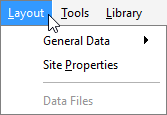
Figure 1‑7 – Layout Menu
General Data
The General Data menu item contains a series of sub-menus including the System, User and User Files sub-menus.
The System sub-menu is used to gain access to the global simulation parameters, such as parameters related to the operation of the steady-state solver and the optimizer.
The User sub-menu is used to gain access to the user-defined variables.
The User Files sub-menu is used to define custom code and user-defined variables.
Site Properties
The Site Properties item allows users to customize the physical input parameters of the plant (Plant Site Properties tab) and the simulation date (Simulation Setup tab). Additional plant information can also be saved under the Plant Information tab.
Data Files
The Data Files menu is only available in Simulation Mode and is used to manage the files used in the active scenario (see Using Scenarios). From this menu you create new datafiles, add existing data files to the scenario or remove data files from the scenario. You can also edit data files, but if the file is used in multiple scenarios, it will change the information in all of them.
Tools Menu
The Tools menu includes items related to the setup and use of a plant model.
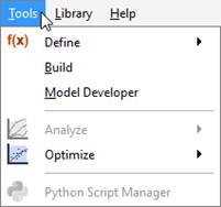
Figure 1‑8 – Tools Menu
Define
Allows you to interactively specify an equation for calculating one of six different layout-wide variables including the Solids Retention Time (SRT) and Food/Microorganism ratio (F/M). In practice, it is found that formulation of the defining equations for these variables is plant specific. The Define feature allows you to interactively specify how these variables are to be calculated for a specific layout.
Build
There is an “auto-build” feature which knows when to build and rebuild model code. However, if users wish to force a model build, it can be done from this menu.
This translates the flow sheet to binary executable code. GPS-X uses a special procedure to convert the graphical images in the drawing board first to a high-level simulation language (ACSL) code and then to a FORTRAN binary executable program.
Analyze
(This feature is available only to those who have purchased the Analyzer module)
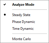
Figure 1‑9 – Analyze Menu
Used to test the ‘model validity’ by conducting sensitivity analyses on selected parameters.
The Analyzer is turned ‘on’ by selecting the Analyze Mode checkbox in the Analyze sub menu, or by clicking on the Analyze button on the toolbar.
With the Analyzer active, four options exist for the analysis:
|
Steady State |
conducts a steady state simulation for different values of independent variable |
|
Phase Dynamic |
calculates state variables at a specified point in time for different values of the independent variable. |
|
Time Dynamic |
conducts a dynamic simulation for each value of an independent variable for a specified time interval. |
|
Monte Carlo |
conducts a Monte Carlo analysis of an independent variable for a specified range and probability distribution. |
Optimize
(This feature is available only to those who have purchased the Optimizer module)
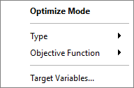
Figure 1‑10 – Optimize Menu
A flexible, dynamic optimization package for evaluating important model parameters. Given appropriate dependent data, and a user-defined objective function, GPS-X can identify an optimal value for a selected model parameter.
The Optimize sub-menu controls the set up and operation of the optimization tools.
In Modelling mode, selecting the Optimize Mode will start a wizard that will set you through the process of setting up the optimization.
In Simulation mode, selecting the Optimize Mode will inform the program that the simulation that is about to be performed should use the optimizer feature.
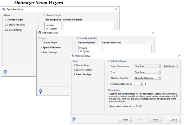
Figure 1‑11 – Optimizer Setup Wizard
An optimizer setup wizard is used for specifying target variables, optimize variables, and optimizer settings. Once these are specified, you must switch to simulation mode where GPS-X automatically creates an input parameter menu with the optimized parameters and creates an output graph of the target variables.
Type
Two options are available from this sub-menu:
|
Time Series |
optimizes based on a set of one or more time series of dependent data |
|
DPE |
(Dynamic Parameter Estimation) – optimizes a moving time window of data for use in on-line model calibration. (This feature is available to those who have purchased the Advanced Tools optional module.). |
The data requirements and form of the objective function depend on the type of optimization being performed.
Objective Function
You have the flexibility of specifying the form of the objective function to use. This sub-menu contains several objective function options including:
|
Absolute Difference |
creates an absolute error form of the objective function. |
|
Relative Difference |
creates a relative error form of the objective function. |
|
Sum of Squares |
creates and absolute sum of squares error form of the objective function. |
|
Relative Sum of Squares |
creates a relative sum of squares error form of the objective function. |
|
Maximum Likelihood |
creates a maximum likelihood from of the objective function. |
In the objective functions, the errors associated with a target variable are the differences between the predicted values and the observed values.
Target Variables
This menu item displays a list of the target variables selected for the optimization. You can use this item to verify the target variable names.
Python Script Manager
This menu item brings up the “Python Script Manager” Window. The Python Script Manager is only available when GPS-X is in Simulation mode. This window is used to edit or run existing Python scripts in GPS-X and create new Python scripts.
Library Menu
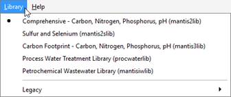
Figure 1‑12 – Library Menu
The library menu is used to select/view which library the current layout used. View the Technical Reference Manual for more information about libraries.
Help Menu
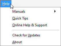
Figure 1‑13 – Help Menu
Manuals
The Manuals menu item contains links to the GPS-X companion literature. Selecting the User’s Guide, Tutorial Guide, Model Developer Guide, and Technical Reference will display the corresponding GPS-X manual in electronic format using Adobe Acrobat Reader.
Quick Tips
The Quick Tips menu item will open a GPS-X Quick Tip. These tips highlight GPS-X features you may be unaware to help you enhance your GPS-X user experience.
Online Help & Support
The Online Help & Support menu will link you to Online Help and Support page of the Hydromantis/Hatch website.
Check for Updates
The Check for Updates menu item will verify that you are using the latest version of GPS-X
About
The About menu item will display information on this version of GPS-X.
Main Toolbar
The buttons are listed below. Not all of the buttons are available in both Simulation and Modelling Modes. For information about the actions that they perform, see the corresponding menu item description in the previous section.
|
|
New Layout |
|
|
Open Layout |
|
|
Save Layout |
|
|
Cut |
|
|
Copy |
|
|
Paste |
|
|
Rotate |
|
|
Mirror |
|
|
Zoom to Selection/Plant |
|
|
Display Labels |
|
|
Define |
|
|
Analyze |
|
|
Optimize |
|
Units: SI/US |
Default Unit Set |
|
|
Data Files |
|
|
Report |
Drawing Board
The drawing board is the large area in the center of the main window. This is where you define your treatment plant process flow diagram. See Creating Model Layouts in CHAPTER 2 for a description of how to do that.
|
|
The Site Properties button can be found in the upper left-hand corner of the drawing board. See Site Properties in CHAPTER 4 for a description of its use. |
Modelling/Simulation Mode
![]()
Figure 1‑14 – Modelling/Simulation Mode Buttons
The Modelling/Simulation Mode button allows the user to switch between the two modes. It also activates the automatic rebuilding of layouts (if applicable).
|
Modelling Mode |
For creating and/or editing models. Users must be in Modelling Mode to draw and change models on the drawing board, define new variables and/or source objects. Any user-defined code (see Customizing GPS-X) must be entered while in this mode. |
|
Simulation Mode |
For using the model and doing analyses. Users must be in Simulation Mode to run the model, create and use scenarios, create and use input and output graphs, and use the analyze/optimize functions. The GPS-X layout drawing board will appear with a grey background when in Simulation Mode. |
Simulation Toolbar
The Simulation Toolbar is only displayed in Simulation Mode. It is at the bottom of the main window.
![]()
Figure 1‑15 – Simulation Toolbar
Simulation Progress Controls
|
|
Start |
Runs the simulation from the beginning. |
|
|
Resume |
If a simulation has been paused, this will resume the simulation from that point. If a simulation has reached it’s ‘Stop Time’, then you can increase that value and then continue the simulation. |
|
|
Pause |
Pause a simulation. |
Steady State
This checkbox controls whether or not to use the steady state solver.
Convergence/Simulation Progress Bar
This progress bar shows either the steady state convergence percentage (grey) or the simulation progress (blue).
![]()
Figure 1‑16 – Convergence/Simulation Progress Bar
Scenario
This menu contains scenario-related commands including the commands to select, create, delete, and show the contents of scenarios. See Using Scenarios section in CHAPTER 8 for more information.
Stop Time/Communication/Delay
This area of the simulation toolbar allows you to edit the stop time, communication interval, and the delay value. These three parameters can be changed interactively as the simulation proceeds.
Click on the label to switch between the three variables.
Stop Time is the amount of time that the simulation will run before stopping. This value is also used to set the maximum time on time series graphs.
Communication interval is the period of time between communication with the model and the graphical interface. This interval affects both the spacing between data points on a graph and updating the model with the values of the input controllers. It can be any positive value greater than zero.
Delay is an artificial delay inserted in the simulation routine, which slows the simulation. For some models, this may be necessary to allow enough time to change controls and observe responses.
Simulation Control
|
|
This menu contains various settings regarding the simulation and some different low-level commands that can be sent to the model. For more information about these options, see the Simulation Control section in CHAPTER 8. |
Reset
|
|
The Reset button can be used to clear all the previous simulation iterations and results. This feature keeps all the layout settings but resets the Initial Conditions . Most people do not need to use this feature because simply starting the simulation over again (by pressing the Start button) will begin the simulation in an adequate place. |