Tutorial 7
Problem Statement
With any model, one of the first exercises to carry out is a sensitivity analysis of the model parameters. There are two reasons for doing so: 1) to validate the model results and 2) to identify parameters to be adjusted during calibration. The former reason should allow the modeler to develop some confidence in the model so that it behaves in an expected manner. For example, increasing the influent flowrate in a membrane filter ultimately results in the increase of mass of hauled sludge in the sludge formation process. The latter reason for performing a sensitivity analysis, parameter identification, is useful because it helps determine the parameters that have the most impact on the model response. We do not want to adjust parameters during a calibration run that have little effect on the model behavior.
After the model is calibrated and verified, sensitivity analyses are useful for other reasons. Mathematical models can be revealing, sometimes allowing us to explore operational strategies that might never have been contemplated otherwise.
In this chapter, you will explore the steady-state and dynamic sensitivity of a basic model.
Objectives
The purpose of this tutorial is to see how we can extract as much information as possible from a GPS-X model. By the end of this tutorial, you should have developed a working knowledge of the Analyzefunctions. This includes setting up and running steady state, phase dynamic, and time dynamic sensitivity analyses. By completing this tutorial, you will also learn how to interpret the results from these simulations.
Setting Up the Layout
The Analyze module is an optional feature of GPS-X. If you have not purchased this module, contact Hydromantis/Hatch for pricing information.
Because this feature requires multiple simulations, for demonstration purposes the work will be carried out on a simple model consisting of a Ground Water influent (Raw Water Sources Group), an Alkali Dosage (Chemical Feed Group), a Lime Softening Tank (Chemical Treatment Group), a Primary Clarifier (Physical Treatment Group) and an Effluent object (Effluent Group).
1. Create a new layout
2. Select the Process Water Treatment Library (procwaterlb) from the library menu (if not already selected).
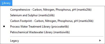
Figure 7‑1- Select Library
3. Create a layout as shown in Figure 7‑2. The layout contains the following objects:
· A Ground Water object from the Raw Water Sources section with the tsstoc model selected
· An Alkali Dosage object from the Chemical Feed section with the alkalifeed model selected
· A Lime Softening object from the Chemical Treatment section with the react model selected
· A Circular Secondary Clarifier object from the Biological Treatment section with the empiric model selected
· A Treated Water object from the Effluent section with the default model selected
4. Connect and label the objects as seen in Figure 7‑2.
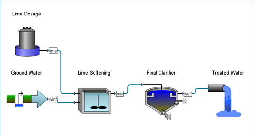
Figure 7‑2- Tutorial 7 Layout
5. Save the layout with the name ‘tutorial-7’.
Setting Up the Analysis Parameters
6. Switch to Simulation Mode.
7. Create a new scenario. Call it ‘Softening’.
8. Change the influent parameters. Access the Ground Water process menu and change:
· Flow > Flow Data > influent flow parameter to 5,000 m3/d
· Flow > Flow Data > flow type parameter to Sinusoidal
9. Change the Alkali Dosage parameters:
· Composition > Feed Chemical Details > chemical parameter to Ca(OH)2
· Composition > Feed Chemical Details > Ca(OH)2 concentration to 30% purity Ca(OH)2
10. Create input controls. Place the influent flow and the alkali flow rate on an input control tab. They are found in the following locations:
· The Influent Flow variable can be found in the Ground Water object Flow > Flow Data menu
· The alkali dosage flow rate can be found in the Alkali Dosage object Flow > Flow Rate Setup menu
Put both parameters on the same input control tab, with the limits of 1,000 – 10,000 m3/d for the influent flow and 0.0 – 2.0 m3/d for the alkali flow
Rename the input tab “Flow Controls”
11. Create output graphs. You will create four different graphs. One for each of:
· Estimated pH (from the Treated Water Output Variables > Water Chemistry Variables form)
· Carbonate Hardness (from the Treated Water Output Variables > Water Chemistry Variables form)
· Total Alkalinity (from the Treated Water Output Variables > Water Chemistry Variables form)
· Turbidity (from the Treated Water Output Variables > Water Chemistry Varibles form)
Use limits of 0-14 for estimated pH, 0-500 mgCaCO3/L for Hardness, 0-400 mgCaCO3/Lfor Total Alkalinity and 0-75 NTU for Turbidity.
Rename the output tab “Effluent Quality”.
12. Auto Arrange the graphs.
13. Save the layout.
Steady-State Analysis
You will now carry out a steady state sensitivity analysis of the lime flowrate on the dependent variables that you have selected for display (pH, Hardness, Alkalinity, Turbidity).
14. Set up the independent variable. Open the settings window for the input controls and change:
· the Type of controller for the alkali dosage flow rate to “Analyze-Step”.
· the Delta value to 0.04. This is the increment that the analyzer will step through from the min to max values.
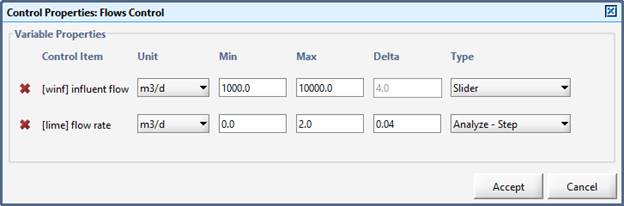
Figure 7‑3- Setting up the Independent Variable
|
|
15. Confirm the analysis type. Click the little arrow beside the Analyze button on the main toolbar (or access it through the main menu’s Tools > Analyze) and confirm that “Steady State” is selected. |
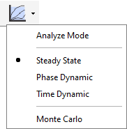
Figure 7‑4- Selecting Analysis Type
16. Switch to Analyze Mode. Click the Analyze button on the main toolbar (or access the Analyze Mode checkbox through the main menu’s Tools > Analyze) and press the Analyze Mode option to turn on analyze mode When in Analyze Mode, the icon on the toolbar will change such that a red checkmark is displayed on the icon.
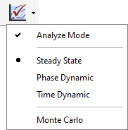
Figure 7‑5- Turn ON Analyze Mode
The status bar at the bottom of the main window will indicate that you are in Analyze Mode and the graphs will change so that the independent variable is the x-axis instead of time.
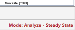
Figure 7‑6- Status Bar Showing "Analyze - Steady State" Mode
17. Run a steady state 0-day simulation.
Observe the effect of an increasing lime flowrate on the effluent pH, Hardness, Alkalinity and Turbidity concentration. Typical results of lime flow rates effect of the effluent Hardness are shown in Figure 7‑7.
Try the analysis using different influent flow rates.
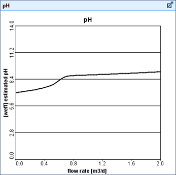
Figure 7‑7- Steady State Analysis Results
Time Dynamic Analysis
You will now carry out a time dynamic sensitivity analysis of the alkali dosage flow rate into the lime softening tank on the dependent variables that you have selected for display (pH, Hardness, Alkalinity, Turbidity).
|
|
18. Change the analysis type. Click the little arrow beside the Analyze button on the main toolbar (or access it through the main menu’s Tools > Analyze) and change the type to “Time Dynamic”. |
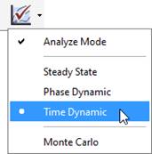
Figure 7‑8- Selecting Analysis Type
19. Switch to Analyze Mode. If you aren’t already in analyze mode (check on the status bar), click the Analyze button on the main toolbar (or access the Analyze Mode checkbox through the main menu’s Tools > Analyze) to turn on the analyzer.
The status bar at the bottom of the main window will indicate that you are in Analyze – Time Dynamic mode. The graphs will have time as the x-axis, just like in the regular simulation mode.
Figure 7‑9- Status Bar Showing "Analyze - Time Dynamic" Mode
20. Set the simulation time to 1-day (with Steady State checked so that the initial conditions are at steady state) and Start the simulation. A mid-simulation result of this sensitivity analysis is shown in Figure 7‑10.
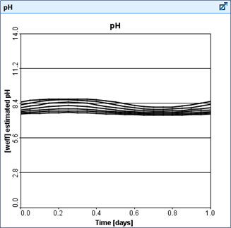
Figure 7‑10- Example of Time Dynamic Analysis Results Mid Simulation
Each successive curve on the various graphs is the result of a dynamic simulation using a specific lime flowrate. Notice in Figure 7‑10 that for increasing values of alkali dosage flow, the effluent pH increase. The effluent pH also fluctuates with time because of the sinusoidal influent pattern. You can change the number of run curves displayed on the graph by going to View > Preferences > Input/Output > Number of runs displayed (analyze/optimize).
Phase Dynamic Analysis
You will now carry out a phase dynamic sensitivity analysis of the lime dosage flow rate into the lime softening tank on the dependent variables that have been selected for display (pH, Hardness, Alkalinity, Turbidity).
21. Select Phase Dynamic from the Analyze drop-down menu.
22. Set the Simulation time to 1-day (with Steady State checked so that the initial conditions are at steady state) and Start the simulation.

Figure 7‑11- Example of Phase Dynamic Analysis
This type of analysis allows you to run the same dynamic simulation as in the previous step. The only difference is in the graphical display. Here the results will be plotted against the analyze variable and not against time. The length of the simulations will set the phase. Typical effluent pH results are shown in Figure 7‑11 for a changing influent lime flow.
In this case, the results are very similar to the Steady Stateanalysis type since the simulation was not very dynamic.
The graph shows the effluent pH after 1.0 day for an influent lime dosage flow rate of 0.0 to 2.0 m3/d (as opposed to showing the steady-state value at time t=0 when carrying out the Steady State analysis).