Tutorial 6
Problem Statement
Automatic process control is well established in many applications ranging from large refineries using multivariate model-based control to climate control of buildings using simple on/off control. Water treatment plants are no exception. The implementation of even basic automatic control should improve performance and save money. In GPS-X, the user can simulate the effects of automatic process control.
To improve the quality of the effluent, as well as minimize chemical costs, you decide to implement an Acid Dosage controller into your system
Objectives
This tutorial will show you how to set up an acid flow PID controller that automatically changes the flow rate of chemical dosages to meet a desired effluent pH.
Using an Automatic Acid Flow Controller
1. Openthe layout completed in Tutorial 2 and save it as ‘tutorial-6’ .
2. Switch to Modelling Mode.
3. Locate the control variable. The pH of the stream leaving the plant through the Treated Water object will be the control variable in this example. We need to know the cryptic variable name (i.e. the internal “short form” variable name used within GPS-X calculations) of this variable so that it can specify it in the controller setup.
Right-click on the Treated Water object and select Output Variables > Water Chemistry Variables. You should see a form like Figure 6‑1.
Hover the mouse pointer over the label for estimated pH and a tooltip should appear. The tooltip has the form label/cryptic. From this we can see that the cryptic name of the variable is phweff. Remember this value for later.
Alternatively, you can right-click on the label for the estimated pH and select “Copy Cryptic Name to Clipboard”. This will store phweff on your computer’s clipboard so that you can paste it into a field later.
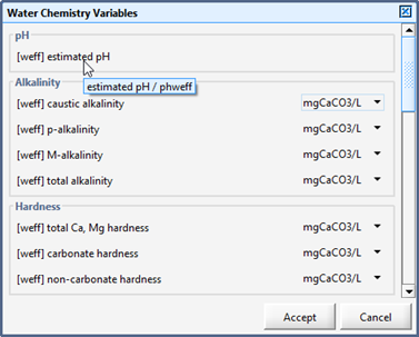
Figure 6‑1- Viewing a Cryptic Variable Name
4. Identify the manipulated variable. The most logical variable for manipulation in this example is the amount of chemical feed being introduced to the system, which in this corresponds to the acid dosage feed rate.
5. Turn on the Acid Feed PID Controller. By default, the Acid Dosage object is set up to feed the system at a constant flow rate, but a PID controller will be setup to dynamically adjust it. Right-click on the Acid Dosage object and go to Flow > Flow Rate Setup. Change the Feed Setup variable under the Flow Rate Setup sub-heading to PID controller.
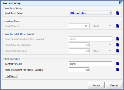
Figure 6‑2- Turn on the PID Controller
6. Define the control variable. At the bottom of the Flow Rate Setup window is a PID Controller sub-heading. Replace the blank in the control variable field with phweff (use CTRL-V to paste the cryptic name if you had previously saved it to the clipboard).
Define the setpoint. Set the setpoint to a pH value of 7.0
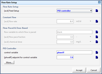
Figure 6‑3- Acid Dosage Controller Definition
7. Define the controller settings. At the bottom of the PID Controller sub-heading (see Figure 6‑3), click the More… button to access the controllers settings (see Figure 6‑4).
· Enter 0.05 days as the controller sampling time (this represents the frequency with which the controller samples the control variable; the effluent pH in this example)
· Enter a value of 20.0 in the field for the proportional gain
· Turn OFF the controller effect on control variable - direct. This means that the manipulated variable, the acid dosage flow rate, will be increased to reduce the control variable, the effluent pH. (A different control loop such as an alkali dosage and the effluent pH would require the controller effect on control variable - direct switch to be turned ON as an increase in the manipulated variable, alkali dosage flow rate, would result in an increase in the control variable, the effluent pH). (i.e. Turn OFF for an inverse relationship and turn ON for a proportional relationship)
· Enter 1.0 m3/d as the maximum pumped flow.
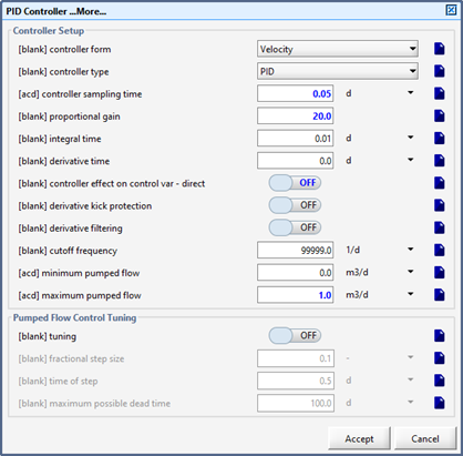
Figure 6‑4- Acid Dosage’s PID Controller Settings
8. Accept the forms.
9. Change the River Water Flow Type to Sinusoidal (found by right clicking on the river water object and going to Flow > Flow Data).
10. Switch to Simulation Mode.
11. Create a new output graph. You will be adding the influent flow rate, the acid dosage flow rate, and the effluent pH to the plot.
Right-click on the River Water object and select Output Variables > Flow. Drag the influent flow variable to a new graph.
Right-click on the Acid Dosage object and select Output Variables > Flow. Drag the Flow variable to the same graph.
Right-click on the Treated Water object and select Output Variables > Water Chemistry Variables. Drag the estimated pH onto the same graph.
12. Edit the graph settings. Change the max y-axis values to 10,000 m3/d, 1.0 m3/d and 14.0 for the influent flow rate, Acid Flow rate and effluent pH respectively. Rename the graph appropriately.
13. Auto Arrange the graph.
14. Rename the output tab “pH Control”
15. Save the Layout
16. Run a 20-day simulation with Steady-State clicked ON
Tuning the pH Controller
We will now address the poorly tuned controller we created in the previous section of the tutorial. It is usually possible to obtain reasonable controller performance by trial and error. In this example, one may conclude that the controller gain is too large. One option for tuning this controller by trial-and-error is as follows:
· Start with a low proportional gain (0.001), high integral time (10 days), and low derivative time (0 days). This creates a sluggish but stable controller.
· Watch how the acid dosage flow rate changes to counteract the effect of a disturbance (e.g. river water flow rate). If it does not react quickly enough, try increasing the proportional gain. Continue to increase the proportional gain until you get a reasonably responsive control effect, but still a stable response.
· If the acid dosage flow rate becomes unstable (wild oscillations) decrease the proportional gain.
· With the proportional effect stable, try decreasing the integral time to increase the performance of your controller.
· If there is too much overshoot, try increasing the derivative time
A simplified understanding of the three elements of a PID controller is: fast, persistent and predictive for the P, I and D terms respectively. Remember that automatic process control is not a simple subject, and it may not be possible to achieve the level of control that you desire.
There are several published approaches for finding good initial tuning constants for PID controllers. One approach is to use the Ciancone correlations (Marlin, 1995[1]) which are included in GPS-X's PID tuning tool. The Ciancone correlations provide the tuning constants given the gain, time constant, and dead time of the process, under the assumption that the process dynamics may be represented with reasonable accuracy by a first-order plus dead time model. In GPS-X's PID tuning tool, the process response to a step change in the manipulated variable is fit to a first-order plus dead time model using least squares (in tuning mode). The Ciancone correlations are then used to determine the appropriate values for the tuning constants.
We will now use GPS-X’s built in PID tuning tool to tune the controller:
17. Create a new scenario. Base the scenario on the Base Model and call it Tuning.
18. Create a new input control tab. Rename this tab ‘pH control’. We will be adding 5 input controllers to this tab.
From the Acid Dosage Flow > Flow Rate Setup menu add the following:
· Feed Setup
· Setpoint for control variable (set limits from 0 to 14)
From the Acid Dosage Flow > Flow Rate Setup > PID Controller More.. menu add the following within the Controller Setup heading:
· proportional gain (set limits from 0 to 50 d)
· integral time (set limits from 0 to 10 d)
· derivative time (set limits from 0 to 10 d)
19. Activate the Acid Dosage flow rate tuning mode.
Browse to the Acid Dosage’s Flow > Flow Rate Setup form. Click on the PID Controller section’s More… button and find the Pumped Flow Control Tuning section.
Turn the tuning switch ON. Drag this variable to the pH control input control tab so that it can be easily turned OFF later.
The fractional step size can be specified on that form and can be a positive or negative value. In this case, set the fractional step size to 0.5.
Accept the More dialog to return to the Flow Rate Setup form.
Now (under the Flow Rate Setup section) change the Feed Setup to Constant Flow. Under the Constant Flow Heading, set the flow rate to 0.2 m3/d.
This fractional step size corresponds to a step in the acid dosage flow rate from 0.2 m 3 /d to 0.3 m 3/d.
Add both Feed Setup and flow rate to the pH Control input controller tab
Acceptthe Flow Rate Setup form.
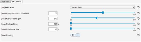
Figure 6‑5- pH Controller Input Controls
20. Double-check that you have the right settings. Select Scenario > Show from the Simulation Toolbar to see all the variables that you have changed in this scenario. You should see a dialog similar to Figure 6‑6.
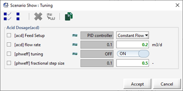
Figure 6‑6- Scenario Show Dialog
21. From the input control tab, turn the pH controller ON by changing the Feed Setup to PID controller and run a 0-day steady state simulation with the newly created scenario.
22. Set the stop time to 10 days and run a simulation with the steady state box checked [2].
The simulation performed in tuning mode is shown in Figure 6‑7. The essential characteristics of a successful tuning mode simulation are:
· It must be started under steady-state, with values of the manipulated (acid flow rate) and controlled (pH) variables representative of normal operating conditions.
· The simulation should last long enough to capture most of the process dynamics (i.e. the simulation should end at steady-state, or be approaching steady-state), and
· The step in the manipulated variable should be large enough to dominate other "noise" that affects the controlled variable (in this case the sinusoidal influent flow pattern).
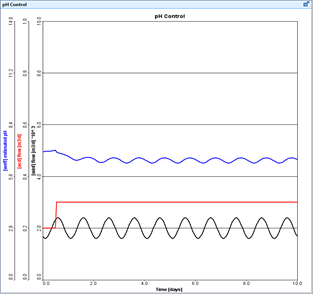
Figure 6‑7- Tuning Mode Simulation
At the end of the simulation, PID tuning constants will be calculated (this may take several seconds) and will appear in the Command Window (see Figure 6‑8).
|
|
The Command Window can be opened by selecting this option from the Simulation Control button on the Simulation Toolbar. Scroll to the bottom of the Command Window for the controller settings displayed in Figure 6‑8. |
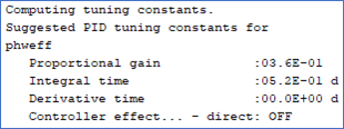
Figure 6‑8- Calculated PID Tuning Constants
23. Create another scenario. Base it on the Tuning scenario (so that it starts with all the variables from that scenario) and call it “pH Control”.
24. Change the input controller values. In the input control tab, set the proportional gain, integral time, and derivative time to the values shown in the Command Window. Also turn OFF the tuning mode.
25. Turn off tunning mode and make sure that the Feed Setup controller is set to PID controller
|
|
26. Transfer the controller values to the scenario. Press the “Transfer controls to scenario” button on the Controls toolbar and add the controller tuning constants to the scenario to store these settings. Pressing Accept will make these the default settings in the pH Control scenario. |
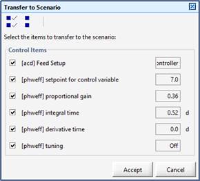
Figure 6‑9- Transfer to Scenario
27. Create an input controller to control the river water flow rate.
28. Save the Layout.
29. Run a 10-day simulation with Steady-State clicked ON. The results shown in Figure 6‑10 were performed using these tuning parameters for the pH controller. The pH setpoint was 7.0 and the influent flow rate was increased to test the performance of the controller under dynamic conditions.
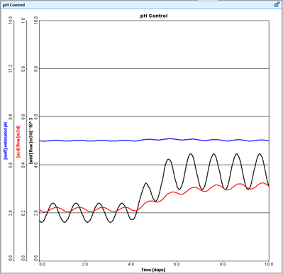
Figure 6‑10- Simulation with pH Controller