Tutorial 1
Introduction
Dynamic process models have great potential for assisting operators, engineers, and managers. However, in the past dynamic models were not used very often because the costs of building models, running simulations, and interpreting the results were too expensive. In order to simplify the modelling process and therefore reduce the cost, you need tools to aid you with the steps in any modelling exercise.
A tool like GPS-X is invaluable as its easy-to-use interface connected to a powerful library of simulation models will greatly reduce the expense of carrying out simulation studies.
There are five major steps in any modelling study:
1. Model construction
2. Model calibration
3. Scenario development
4. Simulation
5. Interpretation of results
In this tutorial, you will develop and simulate a simple steady state model of a clean water system.
Objective
This tutorial covers the following topics:
1. Building a simple plant layout
2. Preparing the source and binary code
3. Running a simple simulation
When you have finished this tutorial, you will be able to build a process layout in the modelling environment and then simulate it in the simulation environment. This provides a supporting basis for the subsequent tutorials where you will learn how to create interactive controls and output graphics.
Building a Simple Plant Layout
After opening a new file in GPS-X:
1. Select the Process Water Treatment Library (procwaterlib) from the Library menu.
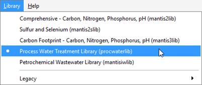
Figure 1‑1- Select Library
2. Locate the Process Table on the left-hand side of the GPS-X window. These icons are used to build a plant layout. Icons represent the unit processes and control points in a layout. The icons are separated into groups of like objects, such as Raw Water Sources, Chemical Feed, Physical Treatment and Disinfection.
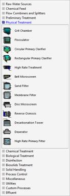
Figure 1‑2- Process Table
The Process Table contains the unit process icons used to construct a treatment plant model. Each icon is identified by process name. The process name is also displayed in a tooltip if you hold the cursor over any object in your drawing board.
We will start by building a simple water treatment plant consisting of 5 objects:
· A River Water Influent
· A Neutralization Tank
· An Acid Dosage
· A Treated Water
|
|
3. Place the River Water Influent object on the drawing board. If the Raw Water Sources group is not selected in the process table, click on the Raw Water Sources group to display the influent process objects. Place the cursor over the River Water influent object. Click on the left mouse button and with the button pressed, drag the cursor to the center of the drawing board and drop the object by releasing the mouse button. The influent object now appears in the drawing board. You can drop as many of these objects as desired by repeating this procedure. For now, drop only one influent object.
|
|
|
4. Select the Membrane Filter icon (Physical Treatment group) and drop it on the drawing board to the right of the influent object.
|
|
|
5. Select the Neutralization Tank icon (Chemical Treatment group) and drop it to the right of the Membrane Filter.
|
|
|
6. Select the Acid Dosage icon (Chemical Feed group) and drop it above the Membrane Filter. |
|
|
7. Select the Treated Water icon (Effluent group) and drop it to the right of the Neutralization Tank.
|
|
|
8. (Optional) Close the Process Table by clicking on the left-pointing arrow at the top-right corner of the Process Table or by going to View > Toolbars > Process Table from the main menu. |
The drawing board should now look similar to Figure 1‑3.
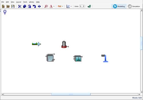
Figure 1‑3- Drawing Board With 5 Unit Processes
|
|
9. Zoom in by using the Locator. This is a simple plant with a large amount of white space on the drawing board and zooming will allow us to see the objects on the drawing board more clearly. The Locator can be used to zoom in on an area of interest while leaving white space for additional objects. The Locator can be accessed by going to View > Zoom. The Locator window will be displayed as shown in Figure 1‑4. |
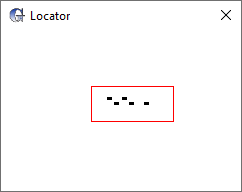
Figure 1‑4- Locator Window
10. Zoom in or out by selecting a region in the Locator window (left click, drag and release). Try selecting an area much larger than the rectangle currently displayed in the Locatorwindow. When you release the mouse button the drawing board is refreshed and the icons on the drawing board appear smaller. Try dragging-out a smaller rectangle around the process units and note the effect in the main drawing board area. You should see an enlarged view like that shown in Figure 1‑5.
|
NOTE: The area in the Locator window represents the total available drawing area. When you drag out a region in the Locator window and release the mouse button the region within the drag rectangle is displayed in the drawing board area, scaled as necessary. Alternatively, the mouse wheel can also be used to zoom in and out on the layout.
|
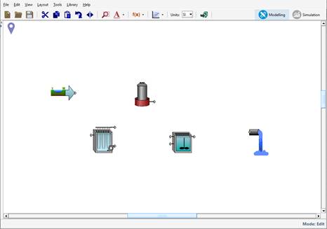
Figure 1‑5- Enlarged Drawing Board Area
|
|
11. Zoom in by using the Zoom to selection/plant. The Zoom to selection/plant button located on the main toolbar will automatically adjust the current level of zoom to fit all objects on the drawing board. |
This functionality can also be used to automatically zoom in on a specific region of the plant. This can be done by clicking and dragging a blue box around the area of interest on the drawing board. Pressing the Zoom to selection/plant button will zoom in on the highlighted area to fill the drawing board.
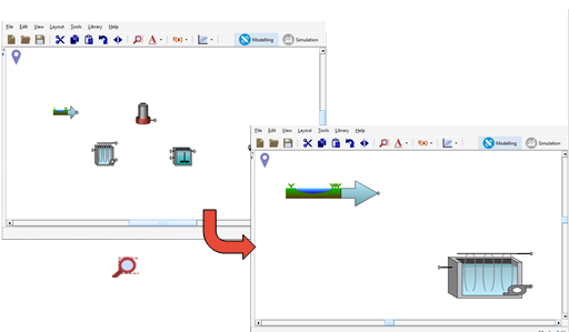
Figure 1‑6- Using Zoom to Selection/Plant to Zoom on a Region of Interest
Press the Zoom to selection/plant button to obtain the enlarged view of the entire plant again.
12. Specify the connectivity between the objects. This is critical in the specification of a flow sheet as all material balances, and therefore the equations which result, are based on the connectivity in the layout. When you specify these connections, remember that the flow lines are directional, i.e., materials flow from the initial point to the terminal point of the flow connection.
|
|
To specify the connectivity between objects, in the drawing board, move the pointer over the influent object connection point. You will know that you are over the connection point when the mouse pointer changes from the default `Windows' arrow to a connecting arrow. When the connecting arrow appears, click to anchor the flow line at this initial point. |
Next, drag the pointer from the influent object to the influent connection point of the membrane filter (top left-hand corner of the icon). When the connecting arrow re-appears, release the mouse button. A connecting pipe will be drawn between the influent object and the membrane filter.
In a similar manner, connect the effluent point from the membrane filter (top right-hand corner of the icon) to the influent connection point of the neutralization tank (bottom left-hand corner of the icon, NOT the chemical input connection point just above on the on the upper-left hand side of the icon).
Connect the effluent point from acid dosage to the chemical input connection of the Neutralization Tank.
Finally, connect the effluent overflow in the neutralization tank (top right-hand corner of the icon) to the Treated Water connection point.
In this example, excess sludge will be wasted from the bottom of the membrane filter (lower right-hand corner of the membrane filter icon). As this model does not consider any downstream processing of the excess sludge, it is not necessary to specify a flow connection from this point (See Figure 1‑7).
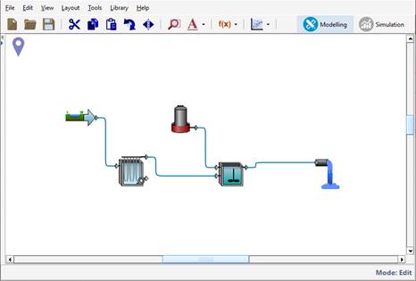
Figure 1‑7- Specifying Connectivity
|
NOTE: GPS-X does not allow invalid flow connections. For example, flows which initiate at the influent of an object and terminate at the influent of a second object are not allowed. GPS-X will disallow an incorrect connection by displaying an invalid sign. If you experience some difficulty in specifying flow connections, you can delete the flow lines by right-clicking on the flow line and selecting Delete Connection |
|
|
13. Rearrange the Connections. The path that a flow line takes from the initiation to termination point can be moved by placing the cursor over the flow line until the mouse icon changes from the default ‘Windows’ arrow to a double ended arrow icon and the connection turns red. Selecting a horizontal segment of the connection will allow you to adjust its path up and down while selecting a vertical segment will allow you to move the flow left and right. |
If you would like to specify a corner point on a flow line, right-click the flow line at the point of interest and select Create Breakpoint from the menu. This will separate the line into two independently moving segments. The break point will stay in place while you modify the other segments.
Try adjusting the flow paths until you are happy with the design of the drawing board. If you would like to revert a connection line back to the GPS-X default path, right-click the connection and select Reset to Auto-Draw from the menu.
14. Show or re-name the labels. There are two types of labels. The unit processes themselves have optional labels and the streams (ie. the flow lines) each have a label. The stream labels are initialized to incremental numbers when a unit process is dropped onto the drawing board.
|
|
In the completed layout shown in Figure 1‑7 there are numbers associated with each of the flow streams. To show/hide these labels on the drawing board, press on the Labels button on the main toolbar to open a dropdown menu where you can specify if you would like the Stream and Object labels to be displayed. Display both the stream and object labels. |
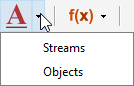
Figure 1‑8- Labels Submenu
Note that the processes that you currently have on the board do not yet have labels, so showing/hiding the Objects label will have no effect at this time.
To change the labels, right-click on an object icon and the process data menu will be displayed. Select the Labels… item from this menu as shown in Figure 1‑9.
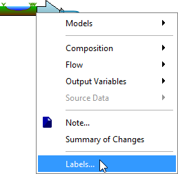
Figure 1‑9- Process Menu Showing Labels Item
New label names can be entered to the form as displayed below. Save these changes by choosing Accept.
If there is a conflict between your label assignments and existing labels, a Labels Error message will be displayed.
Since GPS-X uses label names to construct variable names in the model, it is important to type label names exactly as shown below in Figure 1‑10, Figure 1‑11, Figure 1‑12, Figure 1‑13, Figure 1‑14 for the purposes of this tutorial.
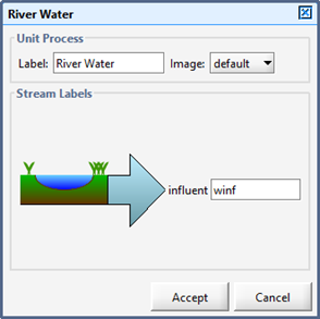
Figure 1‑10- River Water Labels
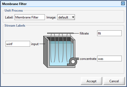
Figure 1‑11- Membrane Filter Labels
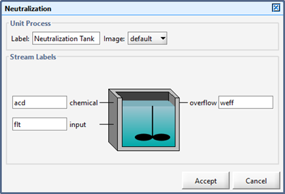
Figure 1‑12- Neutralization Tank Labels
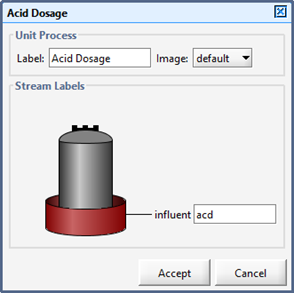
Figure 1‑13- Acid Dosage Labels
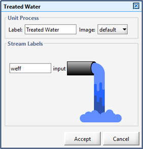
Figure 1‑14– Treated Water Labels
|
NOTE: Variable names in GPS-X models use the connection labels to identify a particular stream (e.g. qwinf for the influent flowrate, and qweff for effluent flowrate in this case). These variable names are displayed on some of the forms you will see as you progress through the tutorial chapters. |
|
|
The plant layout is now ready! If you experience some difficulty in selecting or placing the objects in this layout, you can delete objects from the drawing table by clicking on the object to select it (a light blue box will appear around the object) and then pressing Delete on your keyboard. Alternatively, you can always discard the current drawing board and click on the New button to start over again. |
Selecting Object Models
In the previous section, we selected the basic objects to be modeled in our plant. These objects are the major unit processes and control points only. No mathematical models were assigned to the various objects in the layout.
Each object in the layout has a number of attributes or properties, and each attribute has a certain value. One of the most important attributes for GPS-X objects is the set of equations (or model) that defines the dynamic behavior of that object. Remember to distinguish between an object type and the model for that object as some objects have more than one possible model. Each object is given a default model when it is dropped on the drawing board, but these model choices should be verified and changed if required before proceeding.
15. Verify the influent model. Right-click on the influent icon. The process data menu appears as shown in Figure 1‑15. Verify that the states item is selected under the Models menu...
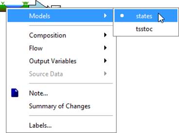
Figure 1‑15- Selecting Models
16. Verify the membrane filter model by repeating this procedure on the membrane filter object. In this case, the only model available should be empiric.
17. Verify the neutralization tank model by making sure that the react model is selected.
18. Verify the Acid Dosage Object model by ensuring the acidfeed model is selected.
19. Verify the Treated Water object model by making sure that the default model is selected. This is the only model available for the treated water.
20. Save the layout. Go to the File menu and select the Save As… menu item. Use the file browser to save the layout to an appropriate directory and with an appropriate name (eg. tutorial-1).
You may have noticed that each object's process menu contains a number of other items for specifying other attributes of an object, such as the Input Parameters, Initial Conditions, andOutput Variables dropdown menus which are available when right-clicking on a process unit on the drawing board.
In this tutorial, we will use the default properties for the objects you have selected with following exceptions:
· The Influent pH
· The Acid Dosage Influent Flow Rate
· The Temperature of Liquid in the Plant
21. Change the influent composition by right clicking on the influent object, move to the Compositionsub-menu and select Influent Characterization. A data entry form called Influent Advisor will be displayed.
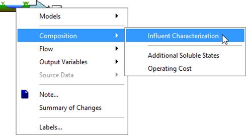
Figure 1‑16- Accessing Influent Characterization
Change the value of the pH variable entry field from 7.0 to 8.0 as shown in Figure 1‑17.
Note that the font of the pH entry field has been changed from blue to black and is now bolded, to indicate that it has been changed from the GPS-X default value.
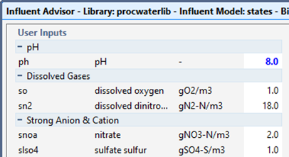
Figure 1‑17- Change Influent Characteristics
22. Change the acid dosage flow rate by right-clicking on the acid dosage object and selecting Flow, Flow Rate setup. A data entry window will open.
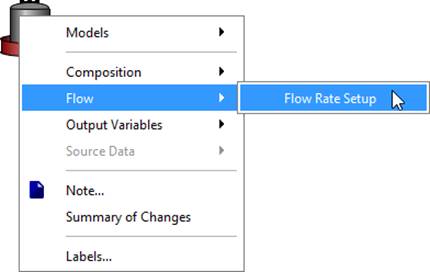
Figure 1‑18- Accessing Operating Parameters
Under the Constant Flow subheading, change the Flow Rate to 0.1 m3/d.
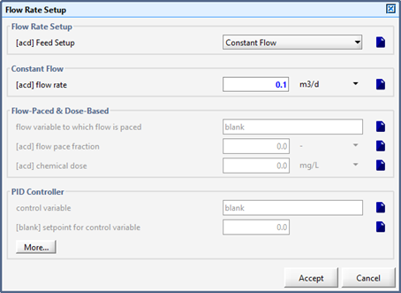
Figure 1‑19- Change the Acid Dosage Flow Rate
Once you have changed the flow rate, press the Accept button.
|
|
23. Once you have completed the layout, you’ll usually want to edit some of the plant wide properties. You can access these properties by pressing the Site Properties button on in the upper left corner of the drawing board. A window will be displayed in which you can specify additional details about the plant and make notes about the model itself. To modify the plant wide properties, selecting the Plant Wide Properties tab of the site properties window. |
Alternatively, you can access this window by going to Layout > Site Properties.
For this example, specify a liquid temperature of 22°C.
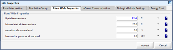
Figure 1‑20– Plant Wide Properties Window
Press Accept to save the changes.
24. To see a list of all the variables in an object that have been changed from the GPS-X default settings, right-clicking on the object and select the Summary of Changes item. Verify the changes made to the influent object.
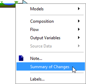
Figure 1‑21– Accessing Summary of Changes
The window that opens will reflect any changes made specifically to the influent object. Currently, it will only show the changes made to the influent pH.
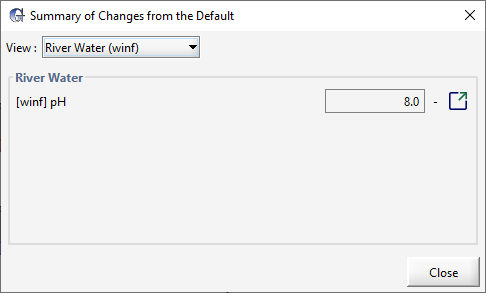
Figure 1‑22– Summary of Changes Made to the Influent Object
On Figure 1‑22 – Summary of Changes Made to the Influent Object, by using the drop-down View menu, you can select other objects on the drawing board to see a summary of the changes made to that object. Selecting the System option will display any changes to the models operating conditions, as well as the plant wide properties. Currently this menu shows the changes made to the liquid temperature.
|
|
The Go to location button can be used to be taken directly to that variable’s entry field to make any additional changes to the variable. The pH variables on the influent object summary of changes window, this will take you to the influent advisor. |
25. Save the layout again by clicking the Save button on the toolbar.
Building A Model
Now that you have built a plant layout, the next step is to translate the layout ‘definition’, into a model that can run simulations.
26. Switch from Modelling Mode into Simulation Mode by pressing the Simulation button (Figure 1‑23) in the upper-right corner of the main window.
![]()
Figure 1‑23- Modelling/Simulation Mode Buttons
This starts the process of compilation and linking, resulting in the creation of an executable model. The time required to complete this process depends on the speed of your workstation, and the complexity of the model.
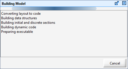
Figure 1‑24- Building model Dialogue
Upon completion of the build step, the Building Model window will automatically close, and you will be left in the Simulation Environment.
Simulation Environment
Once the model has been compiled, GPS-X will present a simulation environment, as shown in Figure 1‑25.
The layout is shown in the lower left-hand corner, the blank area in the upper left-hand corner is for input controllers, and the output area is on the right-hand side of the simulation environment.
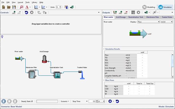
Figure 1‑25- Simulation Environment
Notice that a standard unit process output tab for each unit in the layout (River Water, Acid Dosage, Membrane Filter, Neutralization Tank, and the Treated Water Object) are automatically generated in the output section (Figure 1‑26). These are Quick Display summary tables, which will display output results after simulations are carried out.
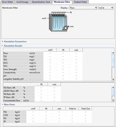
Figure 1‑26– Membrane Filtration Quick Display Panel
You can quickly bring a desired Quick Display panel to the front by double-clicking on the unit process on the drawing board as an alternative to clicking on each individual process tab in the panel.
There are three subdivisions in the Quick Display panel:
1) Simulation Parameters. This sub-heading is used to display important information about the object’s operational parameters specified in Modelling Mode.
2) Simulation Results. This sub-heading provides a summary of the simulation results, highlighting some key characteristics of the influents, effluents and internal conditions
3) Mass Flows. This sub-heading provides a summary of the mass of TSS, COD, TN and TP that can be found in each stream entering and exiting an object.
The Quick Display is not able to have both the Simulation Parameters and the Simulation Results sub-sections open at the same time. To open or close a subsection, click on the sub-section’s header. If you open one of these subsections the other will automatically be closed. For example, opening the Simulation Parameters subsection will close the Simulation Results subsection.
Running A Simulation
Your model is now ready to run a simulation. The controls that you will need to run a simulation are located on the Simulation Toolbar found at the bottom of the screen.
![]()
Figure 1‑27- Simulation Toolbar
|
|
27. Start the Simulation by pressing the Start button on the Simulation Toolbar.
|
Pressing the start button will run a steady state simulation. Once the simulation is complete the tables in the output area will be populated with values.
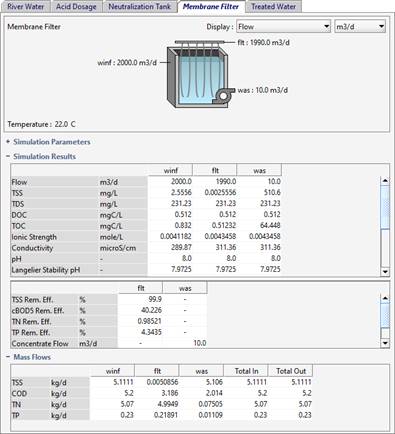
Figure 1‑28- Membrane Filtration Quick Display Panel with Simulation Results
28. Switch between the various Quick Display windows to view the simulation results for each unit process in the layout.
29. Save the Layout. Press the Save button on the main toolbar.