GPS-X Version 8.0
Copyright ©1992-2019 Hydromantis Environmental Software Solutions, Inc. All rights reserved.
No part of this work covered by copyright may be reproduced in any form or by any means - graphic, electronic or mechanical, including photocopying, recording, taping, or storage in an information retrieval system - without the prior written permission of the copyright owner.
The information contained within this document is subject to change without notice. Hydromantis Environmental Software Solutions, Inc. makes no warranty of any kind with regard to this material, including, but not limited to, the implied warranties of merchantability and fitness for a particular purpose. Hydromantis Environmental Software Solutions, Inc. shall not be liable for errors contained herein or for incidental consequential damages in connection with the furnishing, performance, or use of this material.
GPS-X and all other Hydromantis trademarks and logos mentioned and/or displayed are trademarks or registered trademarks of Hydromantis Environmental Software Solutions, Inc. in Canada and in other countries.
ACSL is a registered trademark of AEgis Research Corporation
Python is a registered trademark of the Python Software Foundation.
GPS-X uses selected Free and Open Source licensed components. Please see the readme.txt file in the installation directory for details.

Table of Contents
Introduction to Modelling and Simulation
Benefits of Mathematical Modelling
Influent Wastewater Characteristics
Biological Reactor and Final Settler
GPS-X State Variable Libraries
GPS-X Composite Variable Calculations
Composite Variables in CNIPLIB
Composite Variables in CNPIPLIB
Composite Variables in MANTIS2LIB
Composite Variables Calculated from Non-Modelled States
Influent Objects in CNLIB, CNPLIB, CNIPLIB, CNPIPLIB
Chemical Dosage Influent Object
Influent Objects in MANTIS2LIB
Summary of Aeration Input Parameters
Activated Sludge Biological Models
Activated Sludge Model No. 1 (ASM1)
Activated Sludge Model No. 2 (ASM2)
Activated Sludge Model No. 2d (ASM2d)
Activated Sludge Model No. 3 (ASM3)
New General Model (NEWGENERAL)
Pre-fermenter Model (Prefermenter)
Suggestions for Selecting an Activated Sludge Model
Special Activated Sludge Units
Anaerobic Membrane Bioreactor (Mantis2 and Mantis3 only)
Sequencing Batch Reactor (SBR)
Continuous Flow Sequencing Reactor (CFSR)
High Purity Oxygen (HPO) System
Modelling of Temperature Dependent Kinetics
Toxic Inhibition in IP Libraries
Rotating Biological Contactor (RBC) Model
Submerged Biological Contactor (SBC) Model
Simple Biological Aerated Filter (BAF) Model
Advanced Biological Aerated Filter (BAF) Model
Membrane-Aerated Bioreactor (MABR)
Sedimentation and Flotation Models
Basic Anaerobic Digestion Model
In-line Chemical Dosage Object
Advanced Oxidation Process (AOP)
Tools and Process Control Objects
Feedforward-Feedback Controllers
Operating Cost Model Parameters
Operating Cost Model Output Variables
Calibration of Operating Cost Models
Summary of the Optimizer Settings and Parameters
Appendix A: Maximum Likelihood Method
Appendix B: The Optimizer Solution Report
Statistical Criteria to Evaluate Simulation Results in Wastewater Treatment Modelling
Table of Figures
Figure 4‑1 – Diagram Nomenclature
Figure 4‑8 - MANTIS2LIB - Calculation Procedure for Composite Variables VSS, TSS
Figure 4‑9 - MANTIS2LIB - Calculation Procedure for Composite Variables STKN and TKN
Figure 4‑10 - MANTIS2LIB - Calculation Procedure for Composite Variables STP, XTP, and TP
Figure 4‑11 - MANTIS2LIB - Calculation Procedure for Composite Variables STOC and TOC
Figure 5‑1 - Opening the Influent Advisor Tool
Figure 5‑2 - Influent Advisor Menu
Figure 5‑4 - Selecting the Influent Flow Data Menu
Figure 5‑5 - Influent Flow Data Menu, showing Flow Type Options
Figure 5‑6 - The Influent Models
Figure 5‑7 – MANTIS2 Library BODbased Influent Model Inputs
Figure 5‑8 – MANTIS2 Library Nutrient Fractions for the BODbased Influent Model
Figure 5‑9 - CODstates Influent Model Inputs
Figure 5‑10 - CN Library States Influent Model Influent Stoichiometry Inputs
Figure 5‑11 - CN Library tsscod Model Particulate Inert Calculation
Figure 5‑12 - CN Library tsscod Influent Soluble Components Calculation
Figure 5‑13 - CN Library Acetate Influent Model - Acetate Dose Form
Figure 5‑14 - CN Library Methanol Influent Model Inputs
Figure 5‑15 - Batch Input Menu - Flow Data Model Inputs
Figure 5‑16 – CN Library Organic State and Composite Variables
Figure 5‑17 - CN Library Nitrogen State and Composite Variables
Figure 5‑18 - CNP Library Organic State and Composite Variables
Figure 5‑19 - CNP Library Nitrogen State and Composite Variables
Figure 5‑20 - CNP Library Phosphorus State and Composite Variables
Figure 5‑21 - Accessing the Stoichiometry Parameters in MANTIS2LIB
Figure 5‑22 - Influent Specific Stoichiometric Parameters
Figure 5‑23 - Fixed Stoichiometric Parameters in MANTIS2LIB
Figure 5‑24 - More... Fixed Stoichiometric Parameters in MANTIS2LIB
Figure 5‑25 - Models in COD Chemical Dosage Influent Object
Figure 5‑26 - Accessing Feed Chemical Details Menu
Figure 5‑27 - Selection of Feed Chemical and Set-up of Chemical Properties
Figure 5‑28 - Models in Acid Dosage Influent Object
Figure 5‑29 - Accessing Feed Chemical Details Menu
Figure 5‑30 - Selection of Feed Chemical Set-up of Chemical Properties
Figure 5‑31 - Models in Alkali Dosage Influent Object
Figure 5‑32 - Accessing Feed Chemical Details Menu
Figure 5‑33 - Selection of Feed Chemical and Setup of Chemical Properties
Figure 5‑34 - Models in Nutrient Dosage Influent Object
Figure 5‑35 - Accessing Feed Chemical Details Menu
Figure 5‑36 - Selection of Feed Chemical and Setup of Chemical Properties
Figure 6‑1 - Aeration Setup Form in Operational Form
Figure 6‑2 - General Aeration Setup > More... Form
Figure 6‑3 - Diffused Aeration Setup > More... (Part 1)
Figure 6‑4 - Diffused Aeration Setup > More... Form (Part 2)
Figure 6‑5 - Physical > More... Form within an Object
Figure 6‑6 - Physical Environment Settings (Layout-Wide Settings)
Figure 6‑8 - Predefined air delivery system
Figure 6‑9 - Default curve for diffuser head loss
Figure 6‑10 - ASM3 Model Processes
Figure 6‑11 - General Reaction Pathway
Figure 6‑12 – Schematic Diagram of the prefermenter Model
Figure 6‑13 - GPS-X Membrane Bioreactor Objects
Figure 6‑14 - Membrane Bioreactor Model Structures
Figure 6‑15 – Physical – Membrane Forms
Figure 6‑16 – Membrane Operational Parameters Menu
Figure 6‑17 - Membrane Output Variables Menu
Figure 6‑18 - MBR Cake Variables Menu
Figure 6‑19 – Anaerobic MBR Physical Parameters Menu
Figure 6‑20 - Regular SBR - Operation Cycle Parameters
Figure 6‑21 - Advanced SBR Operational Parameter
Figure 6‑22 - Manual Cycle Operational Parameters
Figure 6‑23 - Oxidation Ditch Recirculation Mode Settings
Figure 6‑24 - 2-D Greyscale Oxidation Ditch Output - Dissolved Oxygen
Figure 6‑25 - Continuous Flow Sequencing Reactor Recirculation Settings
Figure 6‑26 - Continuous Flow Sequencing Reactor Rotating Aeration Bridge Setting
Figure 6‑27 - Continuously Flow Sequencing Reactor Additional Aeration Controllers
Figure 6‑28 - Schematic of High Purity Oxygen (HPO) System
Figure 6‑29 - Typical Outputs from the Energy Balance Model for Temperature Estimation
Figure 6‑30 - Typical Outputs for the Oxygen Transfer Rate
Figure 6‑31 - Variation of Nitrifier Kinetic Parameter Values with Temperature
Figure 6‑32 – Toxic Inhibition Menu
Figure 7‑1 - Conceptual Diagram of the Tricking Filter Model
Figure 7‑2 - Physical Dimensions of the Tricking Filter
Figure 7‑3 - Integration of Soluble Components
Figure 7‑5 - Mass Transport Parameters
Figure 7‑6 - Physical Dimensions of the Trickling Filter
Figure 7‑7 - Tricking Filter Output Variables
Figure 7‑9 – Conceptual Diagram of the RBC Model
Figure 7‑10 - Physical Dimensions of the RBC
Figure 7‑11 – Physical Dimensions of the RBC (More…)
Figure 7‑12 – Physical Dimension of the SBC
Figure 7‑13 - Physical Dimensions of the SBC (More...)
Figure 7‑14 - Simple BAF Model Configuration
Figure 7‑15 - Simple BAF Model Operational Parameters Menu
Figure 7‑16 - Simple BAF Model Operational Parameters Menu (More...)
Figure 7‑17 - Advanced BAF Physical Parameters
Figure 7‑18 - BAF Operational Parameters
Figure 7‑19 - More Advanced BAF Operational Parameters
Figure 7‑20 - Upflow and Downflow Denitrification Filter Objects
Figure 7‑21- Hollow Fibre Membrane Aerated Bioreactor object
Figure 7‑22 - MABR biofilm structure, showing diffusion of soluble components
Figure 7‑23 - MABR Physical Parameters Menu
Figure 7‑24 - MABR Operational Menu
Figure 7‑25 - MABR Operational Menu
Figure 7‑26 - MABR Performance Variables Menu
Figure 7‑27 - MABR Performance Variables Menu
Figure 7‑28 - MABR Performance Variables Menu
Figure 8‑1 - One-Dimensional Sedimentation Model
Figure 8‑2 - Solids Balance Around the Settler Layers
Figure 8‑3 – Settling Velocity vs. Concentration
Figure 8‑4 – Load Distribution into Settler
Figure 8‑5 – Circular Settler Shapes
Figure 8‑6 - Layered Flotation Model
Figure 8‑7 – Physical Parameters for the DAF Unit
Figure 8‑8 - Operational Parameters for the DAF Unit
Figure 8‑9 – Flotation Parameters for the DAF Unit
Figure 9‑1 – Operational Parameters Form – Continuous Model
Figure 9‑2 – Operational Parameters Form – Massbalance Model
Figure 9‑3 - Filter Parameters
Figure 10‑1 - Schematic Diagram of the Anaerobic Digestion Model
Figure 10‑2- General Reaction Pathway
Figure 10‑3 – Parameters Menu for the Anaerobic Digester
Figure 10‑4 - Physical Parameters
Figure 10‑5 –Operational Parameters
Figure 10‑6 - Influent Parameters (Basic Digester Model)
Figure 10‑7 – Effluent Parameters (Basic Digester Model)
Figure 10‑8 - pH Solver Set up
Figure 10‑9 - Kinetic Parameters
Figure 10‑10 - Stoichiometric Parameters
Figure 10‑11 - Simplified ADM1 Material Flow Design
Figure 10‑14 - Reactor Parameters for UASB/EGSB Reactor
Figure 10‑15 - Reactor Parameters Input Form
Figure 11‑1 - Pumping Station Menu
Figure 11‑2 - In-line Chemical Dosage Object
Figure 11‑3 - Removal as a Function of P Concentration
Figure 11‑4 – Dosage Controller Parameters
Figure 11‑6 - Typical Application of Struvite Recovery Reactor
Figure 11‑7 - Typical Process Outputs for Struvite Reactor
Figure 11‑8 - Typical Outputs for Solid Bed Volume and Expansion for Struvite Recovery Reactor
Figure 11‑9 - Breakpoint Chlorination [3]
Figure 11‑10 - Dewatering Object Models
Figure 11‑11 - Operational Menu for Empiric Model
Figure 11‑12 – Belt and Disc Microscreen Objects
Figure 11‑14 - Plot of Calibrated Settleability Model
Figure 11‑15 - Operational Menu for High-Rate Treatment Model
Figure 11‑16 – Operational Menu for High-Rate Treatment Model
Figure 11‑17 - Output Variables Menu in High-Rate Treatment Model
Figure 11‑18 - Solids Removal Efficiency Output Variable Form
Figure 11‑19 - High-Rate Treatment Performance Parameters Output Variables Form
Figure 11‑20 – Custom Interchange Macro
Figure 11‑21 - Inputs for System Curve Definition – Static Head
Figure 11‑22 - Inputs for System Curve Definition - Dynamic Head
Figure 11‑23 - Pump operating point based on pump and system curves
Figure 11‑24 - Pump curves at different pump speeds
Figure 11‑25 - Pump Characteristics Curve - Pump Speed for Pump Curve
Figure 11‑26 - Pump Characteristic Curve Inputs
Figure 11‑27 - Typical Output from a Fixed Pump Speed
Figure 11‑28 - Typical Outputs for Variable Speed Pump
Figure 11‑29 – Operating Cost Output Menu
Figure 12‑1 - pH Model Set up Menu
Figure 12‑2 – Component Control Form
Figure 12‑3 – Sample pH Outputs
Figure 12‑4 – Signal Flow Diagram for the lowpass Model
Figure 12‑6 - Input Form for the Scheduler Model
Figure 12‑7 - Input Form for Setting Duration of Each Phase
Figure 12‑8 - Input Form for Setting the Value of Control Variable in Each Phase of a Sequence
Figure 13‑1 – General Operating Cost Parameters Form
Figure 13‑2 – Input menu for seasonal price model
Figure 13‑3 - Operating Cost Menu
Figure 13‑4 - Layout Operating Cost Display Form (total for all objects)
Figure 13‑5 - Object-Specific Operating Cost Display Form
Figure 14‑1 – Form Containing the Simplex Method Constants
Figure 14‑2 – Optimizer Form Containing the Termination Criteria Settings
Figure 14‑4 - Bottom of Optimizer Form
Figure 15‑1 – Typical Time Series Plot of Predicted and Measured Data
Figure 15‑2 - Statistical Analysis Set up Menu for Data Type, Output Plots and Table
Figure 15‑3 - Summary of the Statistical Measures Calculated for a Time Series Dataset
Figure 15‑4 - Predicted vs. Measured Data Plot
Figure 15‑5 - Histogram of Standardized Residuals
Figure 15‑6 - Residuals Plotted against the Observed Data
Figure 15‑7 - Residuals Plotted against Simulation Time
Figure 15‑8 - Real Time Clock Parameters
Figure 15‑9 - Steady State Parameters
Figure 15‑10 - More Steady-State Parameters
Figure 15‑11 – Integration Methods
List of Tables
Table 3‑1 - Comprehensie Model (MANTIS2LIB) Library State Variables
Table 3‑2 - Comprehensive Model (MANTIS2SLIB) Library State Variables
Table 3‑3 - Carbon Footprint (MANTIS3LIB) Library State Variables
Table 3‑4 – Carbon – Nitrogen Library (CNLIB) State Variables
Table 3‑5 – Industrial Pollutant (CNIPLIB) Library State Variables
Table 3‑6 – Carbon – Nitrogen – Phosphorus (CNPLIB) Library State Variables
Table 3‑7 – CNP Industrial Pollutant (CNPIPLIB) Library State Variables
Table 4‑1 – Example Composite Variable Calculations
Table 4‑2 – CNLIB BOD, COD, and TSS Composite Variables (All Models)
Table 4‑3 – CNLIB Nitrogen Composite Variables – MANTIS Model
Table 4‑4 – CNLIB Nitrogen Composite Variables – ASM1 Model
Table 4‑5 - CNLIB Nitrogen Composite Variables - ASM3 Model
Table 4‑6 - CNPLIB BOD, COD, and TSS Composite Variables
Table 4‑7 - CNPLIB Nitrogen Composite Variables - MANTIS Model
Table 4‑8 - CNPLIB Nitrogen Composite Variables - ASM1 Model
Table 4‑9 - CNPLIB Nitrogen Composite Variables - ASM2d Model
Table 4‑10 - CNPLIB Nitrogen Composite Variables - ASM3 Model
Table 4‑11 - CNPLIB Nitrogen Composite Variables - NEWGENERAL model
Table 4‑12 - CNPLIB Phosphorus Composite Variables - ASM1/MANTIS Models
Table 4‑13 – CNPLIB Phosphorus Composite Variables – ASM3 Model
Table 4‑14 - CNPLIB Phosphorus Composite Variables - ASM2d Model
Table 4‑15 - CNPLIB Phosphorus Composite Variables - NEWGENERAL Model
Table 4‑16 - Stoichiometry Parameters used in Estimation of Composite Variables
Table 4‑17 - Access Menus for Different Stoichiometry Parameters in MANTIS2LIB
Table 5‑2 - State Variables Used in Each Biological Model Included in CNLIB and CNIPLIB
Table 5‑3 – State Variables Used in Each Biological Model included in CNPLIB and CNPIPLIB
Table 5‑4 - Influent Objects in MANTIS2LIB
Table 5‑5 - Alkali Chemicals and Affected States in the Feed
Table 5‑6 - Nutrient Chemicals and Affected States in the Feed
Table 6‑1 – Example Model Matrix (Wentzel et al., 1987a)
Table 6‑2 – Model Processes in GPS-X
Table 6‑3 - Settings of MBR Operating Modes
Table 6‑5 – GPS-X MBR Model – Default Parameter Values
Table 6‑6 – Calibration Suggestions
Table 6‑7 - Library-specific Algorithms for Empiric Pond Model
Table 6‑8 – Heat Transfer Terms with Equations for Estimation
Table 6‑9 – Parameters for the Temperature Model
Table 8‑1 – Sedimentation Model: Input-Output Summary
Table 10‑1 – ADM1 State Variables Set on the ADM1 “Influent” Parameter Menu
Table 10‑2 – ADM1 State Variables Set in the Influent Object
Table 11‑1 - Chemeq Parameters
Table 11‑2 - Sample Pump Characteristics
Table 14‑1 - Summary of How to Use the Statistical Tests
The purpose of this chapter is to provide a basic introduction to modelling and simulation. This chapter will serve to establish the basic definitions for terms that will be used throughout the technical reference. In addition, emphasis will be placed on the advantages of simulation.
When speaking about modelling and simulation, the following terms are often used:
· System
· Experiment
· Model
· Simulation
|
A system is a set of interdependent components that are united to perform a specified function. |
In a general sense, the notion of a system may be defined as a collection of various structural and non-structural elements which are interconnected and organized to achieve some specified objective by the control and distribution of material resources, energy and information. (Smith et al., 1983)
One of the basic aspects of a system is that it can be controlled and observed. Its interactions with the environment fall into two categories:
1. Variables generated by the environment that influence the behaviour of the system (called inputs).
2. Variables that are determined by the system that in turn influence the behaviour of the environment (called outputs).
Accordingly, a system is a potential source of data in that inputs can be defined and observation of the behaviour of the system can be made.
An experiment is the process of extracting data from a system through manipulation of the inputs.
Experimentation is probably the single most important concept of a system; for it is through experimentation that we develop a better understanding of it. Experimentation implies that two basic properties of a system are being used:
1. Controllability, and
2. Observability
To perform an experiment implies the application of a set of external conditions to the inputs of a system (i.e. the accessible inputs) and observe the reaction of the system by recording the behaviour of the outputs (i.e. the accessible outputs). This is where some of the advantages of a system begin to appear. One of the major advantages of experimenting with a "simulated" system as opposed to the "actual" or "real" system, is that real systems are usually under the influence of a large number of additional inaccessible inputs (i.e., disturbances) and that a number of useful outputs may not be available through measurement (i.e., they are internal states of the system).
One of the major motivations for simulation is that in the simulation world, all inputs and outputs are accessible. This allows the execution of simulations that lie outside the range of experiments that are applicable to the real system.
|
A model is an abstraction of a system |
One definition of a model is: A model is an approximation of a system to which an experiment can be applied to answer questions about the system.
A model does not imply a computer program. We should be clear to distinguish between a model and a computer program. A model could be a piece of hardware or simply an understanding of how a system works. Models are often coded into computer programs.
Modelling means the process of organizing knowledge about a given system. By performing experiments, knowledge about a system is gathered. In the beginning the knowledge is unstructured. By understanding the cause and effect relationships and by placing observation in both a temporal and spatial order, the knowledge gathered during the experiment is organized. Thus, the system is better understood by the process of modelling.
|
Simulation is to a model what experimentation is to a system |
Again, many different definitions exist for the term “simulation”. One of the simplest definitions is: A simulation is an experiment performed on a model Again, this does not imply that the simulation is performed on a computer; however, the vast majority of engineering simulations are performed using a computer program. A mathematical simulation is a coded description of an experiment with a reference point to the model to which this experiment is to be applied. The goal is to be able to experiment with models as easily and conveniently as with real systems. It is desired to be able to use the simulation tools as easily as a control chart in the operation of a facility.
While the scientist is normally happy to observe and understand the world, that is, creating a model of the world, the engineer (applied scientist) wants to modify it to his/her advantage. While science is analysis, the essence of engineering is control and design. Thus, simulation can be used for analysis and for design.
Except by experimenting with the real system, simulation is the only technique available for the analysis of arbitrary system behaviour. The typical scenario of scientific discovery is as follows:
1. Perform an experiment on the real system and extract data to gather knowledge (understanding of the cause and effect relationship of the real world).
2. Postulate a number of hypotheses related to the data.
3. Simplify the problem to help make the analysis tractable.
4. Perform a number of simulations with different experimental parameters to verify that the simplifying assumptions are justified.
5. Analyze the system, verify the hypotheses and draw conclusions
6. Simulations are performed to draw conclusions.
A wide variety of simulation tools are available to help you in this task. Assuming the reader is particularly interested in the dynamic modelling of wastewater treatment, the tools appropriate for this task are emphasized.
The process of dynamic modelling of facilities involves the solution of thousands of coupled nonlinear ordinary differential equations. The formulation and solution of this type of problem is facilitated through the use of Continuous Simulation Languages (CSL). CSLs date back to the late 1960s when IBM introduced the language called CSMP (Continuous System Modelling Program). Of the number of very specialized simulation languages that are available, GPS-X uses ACSL for conducting simulations.
Mathematical models assist in developing a thorough understanding of the behaviour of a system and in evaluating various system operating strategies. A proposed system can be evaluated without building it. A costly or unsafe system can be experimented with by using a model rather than disturbing the real system.
One of the most important ways to check the operation of a wastewater treatment plant, the consistency of the analytical procedures and the integrity of the mathematical model is to perform mass balances around the system for the different compounds. This task is not always simple as components transform into other substances, bacterial cells grow, respire and decay.
With regard to the organic substances, a commonly measurable parameter is the Chemical Oxygen Demand (COD). We could measure organic carbon as Total Organic Carbon (TOC) in the plant, but we would miss the fraction which was removed in the form of CO2 gas after oxidation. It is difficult to determine the oxygen requirement based on TOC, as different substances require different amounts of oxygen depending on their chemical composition. The influent wastewater is truly a non-homogenous mixture in this respect.
We could measure the 5-day Biochemical Oxygen Demand (BOD5) and suspended solids as most plants in North America do. Suspended solids have the same problem as TOC with respect to oxidation. BOD5 seems to give relevant information, but it is inappropriate for continuous monitoring, and the accuracy of the results is not comparable to other analytical methods. BOD5 measures only the part of organics which were used for respiration in the BOD test during 5 days, and does not give information about the amount converted into bacterial cells. Ultimate BOD (BODu) corrects this problem but the analytical time and sometimes the accuracy is unacceptable. The BOD test completely ignores a very important fraction of the influent wastewater (inert particulates), which contributes in a major way to excess sludge production.
COD overcomes the above-mentioned problems. It can be automated and measures all organic fractions of the wastewater. The sludge COD can also be easily determined. COD measures all organics in oxygen equivalent; that is the electron donating capacity of the organic matter. This way it provides a direct link between organic load and aeration requirement. The yield constant is truly constant only if expressed in COD units. Mass balance is easy to establish with COD in a non-nitrifying plant: in steady-state, the influent COD must equal the effluent COD plus the COD of the wasted sludge, plus the oxygen consumed in the degradation of organic matter.
It is for this reason that the International Association on Water Quality (IAWQ) committee selected and endorses the use of COD as a measure of organic parameter in simulation of activated sludge plants.
For modelling purposes, each unit process/operation is represented by a process model (mathematical model) that reflects the dynamic behaviour of that particular process. One of the main features of GPS-X is that it is model-independent, meaning that GPS-X is not limited to a specific process model. Accordingly, a variety of modelling approaches (process models) are available within GPS-X to handle a specific unit operation or unit process. For example, the activated sludge process can be modelled using any one of the following GPS-X activated sludge process models:
· IAWQ Task Group models of the activated sludge process (Henze et al.,1987a; Henze et al., 1994; Henze et al., 1998)
· The general (bio-P) model (Dold, 1990, Barker and Dold, 1997)
· Extended IAWQ (Mantis), described in Mantis Model (MANTIS) section of Chapter 6)
· Comprehensive plant-wide model developed by Hydromantis (Mantis2/Mantis3)
Consequently, a general calibration/verification approach to GPS-X must be broadly defined. The calibration requirements of individual process models are established based on the nature of each model (i.e., its mechanistic basis). Alternatively, modellers may need to refer to the original literature reference to assess the calibration requirements of a particular model in more detail.
Each calibration/verification study follows the same general principles. Accordingly, the purpose of this section is to provide some guidelines pertaining to the calibration of the models to full-scale wastewater treatment plants. The most popular process models have been selected for illustration purposes, including the IAWQ Task Group Activated Sludge Model No. 1 (Henze et al., 1987a) and layered settler model developed by Hydromantis (Takács et al., 1991).
In general, modelling of large-scale wastewater treatment plants requires that an extensive number of plant and model parameters be assessed. Many parameters can be measured directly, while others are based on experimental data taken from the literature. Those parameters that cannot be measured directly or estimated from the literature are usually determined using nonlinear dynamic optimization techniques based on actual plant records and/or experimental data collected at the plant or in the lab. It is recognized that the reliability of the calibrated model degrades with increasing numbers of mathematically optimized parameters.
Data requirements fall into one of the following categories:
1. Physical plant data, including: Process flow sheet (flow lines, channels, recycle lines, by-passes, etc.); Flow pattern (plug flow, Continuously Stirred Tank Reactor (CSTR), etc.); Sludge collection and withdrawal locations (location, how? when? etc.); Dimensions of the various reactors (length, width, depth).
2. Operational plant data, including: Flow, Control variables (independent variables), and Responsive variables (dependent variables).
3. Influent wastewater characteristics, including: Basic water quality parameters, influent organic fractions, and influent nitrogen fractions.
4. Kinetic and stoichiometric model parameters for organic, nitrogenous and phosphoric compounds and settling parameters (primary and secondary).
5. Some of these data and/or parameters vary in the course of a day (i.e. subject to dry-weather diurnal variations or during a storm even), while others remain relatively constant.
Elements of this data group are generally easy to obtain from plant blueprints and operation manuals. It should be remembered that the physical volume of a reactor is only an approximation of the active or operational volume of the unit. In a well-designed system the effect of dead-space and hydraulic short-circuiting is normally minimal. In other cases it may be necessary to determine the true hydraulic characteristics of a particular unit process, as in the case of a quasi-plug flow aeration tank. In this case, a dye-test is normally required, as the number of CSTRs becomes a model parameter.
The General Purpose Simulator can handle practically any flow scheme. Based on our experience it is very important to identify as closely as possible the hydraulic characteristics of a plant, including plant by-passes, overflows, flow splits and combiners, proportional, constant or SRT driven sludge wastage, etc. Parallel trains, multiple units and plug flow systems are easily simulated, but should be simplified where possible (unless the required supporting data required for calibration is available).
This is an important data group. For example, if the aeration capacity is not known (or cannot be estimated from the aerator power or other means), then the correct dissolved oxygen (DO) level can be set by either changing the KLa or some stoichiometric or kinetic parameters (yield coefficient, growth rate, etc.). This makes the correct estimation of those parameters difficult. Similarly, model parameters having a strong effect on the aeration tank Mixed Liquor Suspended Solids (MLSS) are difficult to estimate when the wastage rate is not known.
MLSS, Volatile Suspended Solids (VSS), COD of the mixed liquor, DO, and Oxygen Uptake Rate (OUR) are required to calibrate the activated sludge portion of the model. Refer to above section (p. 22) for a discussion on the importance of COD for this chapter (Why COD is Important to Know). In general, the stoichiometry of the mixed liquor (% VSS and COD/MLSS) is relatively constant over time and can be assessed occasionally during the course of a calibration/verification study, e.g., on a monthly or bi-weekly basis. However, the other parameters are generally dynamic, following the diurnal patterns of the plant.
It is important to be able to perform a solids mass balance around the system. Accordingly, the sludge blanket height (and preferably the solids concentration profile) and underflow solids concentration are required to calibrate the settler portion of the model.
Water quality constituents such as BOD5 (inhibited), Total Suspended Solids (TSS), Total Kjeldahl Nitrogen (TKN), ammonia (NH3) and nitrates (NO3) are necessary for the calibration of the various unit processes. For example, BOD (in lack of COD) is used to calibrate and verify the carbonaceous component of the IAWQ activated sludge model, while suspended solids measurements can be useful in identifying the settling parameters of Hydromantis' layered settler model. The nitrogenous compounds are needed to calibrate the nitrification-denitrification component of the model.
Basic influent wastewater characteristics such as BOD5, BODu, COD, TSS, VSS, and TKN are important to know in that they allow us to establish mass balances across the system. The biochemical oxygen demand (BOD) provides only partial information on the influent organic load (see Why COD is Important to Know). COD measurements are not readily available in some wastewater treatment plants. In this case, the BOD5/BODu ratio can better estimate the influent organic load. Suspended solids, influent VSS and BOD together, can be used to determine the different influent organic fractions, which are critical for the proper use of the IAWQ activated sludge model, as discussed in GPS-X Objects. Influent TKN is generally more useful than ammonia concentration alone
The IAWQ activated sludge model contains a large number of stoichiometric and kinetic parameters, which describe the degradation of organic matter in the activated sludge process (Henze et al., 1987a). Some of the analytical tests are laborious and are not discussed here. Many of the default model parameters can be used with a high degree of confidence. Site-specific model parameters include the maximum growth rate and the yield coefficient of the heterotrophs. If the data described in the previous sections are known (e.g., sludge wastage rate and wastewater influent fractions), it is relatively easy to optimize the maximum growth rate and yield coefficient of the heterotrophs to match the measured MLSS, sludge production, and oxygen uptake rate.
Based on our experience, the most important parameter to calibrate in the IAWQ model is the autotrophic growth rate. It is possible to calibrate this parameter using field ammonia and nitrate data, if:
1. The plant is not overloaded, i.e. the plant is at least partially nitrifying; or
2. The plant is not seriously under loaded. In such a case, almost any value of the growth rate constant (typically between 0.2-0.5 d-1) will provide complete nitrification.
The autotrophic growth rate is easier to identify in a partially nitrifying plant. Process start-up data (i.e., corresponding to a slowly developing nitrifier population) can sometimes be used. Laboratory testing (oxidation of an ammonia spike) is also a possibility.
The settling velocity function in Hydromantis' layered settler model contains five parameters, which have to be determined separately for the primary and the secondary clarifiers. A preliminary version of the model is described in detail elsewhere (Takács et al., 1991). The model is based on the use of a unified settling velocity equation described in the chapter on sedimentation and flotation models. The parameters of the settling velocity equation can be estimated from a combination of experimental and numerical procedures.
A short summary of the proposed experimental procedures is given below for each parameter:
· Minimum solids attainable – In general, this parameter for final settlers is usually less than 10mg/L. For most plants, xmin will be close to zero. A sludge sample is allowed to settle for about two hours. The suspended solids concentration of the supernatant is measured and equated to xmin. Alternatively, xmin can be said to be equal to the suspended solids concentration take from the final settler under dry-weather flow conditions, when the hydraulic load to the plant is minimal.
· Maximum floc settling velocity parameter - Dilute the activated sludge to 1 2 g/L, measure the settling velocity of large individual floc particles in a batch test. In general, no floc particle will settle faster than the settling velocity of individual floc particles under quiescent conditions.
· Vesilind zone settling parameters – These two parameters give the settling velocity of the sludge in the hindered settling zone (exponential portion of the curve). They can be determined through a series of column tests (Vesilind, 1968).
· Flocculant settling parameter – If all the above settling parameters are known, then this one is generally easy to estimate by fitting the simulated effluent suspended solids simulations to observed data.
Alternatively, settling velocity model parameters can be estimated using a time-series of influent and effluent (overflow and underflow) suspended solids. The non-linear parameter optimization procedure available in GPS-X can be used effectively in this particular case.
In an ideal case all the physical, operational and influent parameters are known for the given wastewater treatment plant, while some of the most important kinetic, stoichiometric and settling parameters are experimentally determined. In such a case the modeller estimates the missing parameters using defaults at the beginning, then modifying those which need adjustment and observing the response of several system output variables.
It is possible to start with a steady-state calibration, i.e., taking the dry weather days from a daily log of the treatment plant and optimizing for the average of these values. Averages, which contain high flow periods (typical monthly or yearly averages), should not be used for steady-state calibration.
Dynamic calibration should follow with typical diurnal data or selected high disturbance (storm flow) events. The larger the scale of the disturbance between reasonable limits, the more sensitive the calibration procedure will be. Hydraulic shocks are usually ideal for settler calibrations, while diurnal data, process start-up, or recovery is better for calibration of organic degradation and nitrification.
One fully documented event gives reasonable confidence for the given conditions (flow, temperature, influent composition, etc.). If the model is to be used under varying conditions, the above procedure has to be repeated accordingly (i.e., winter, summer, dry weather, wet weather, etc.). Verification means simulating a dynamic event with a given calibrated set of parameters, without modifying those, and finding reasonable accordance of simulated data with the measurements.
A few or several may be missing from the physical, operational and influent group. This does not make calibration/verification impossible, as the interdependencies in a treatment plant are complex and default values are relatively well known. Reasonable estimation of unknown parameters is sometimes possible. In the case of underflows, the solids mass distribution between the aeration tank and the settler depends largely on the recycle flow. Knowing aeration tank MLSS and underflow concentration (maybe sludge blanket height), the missing value can be recreated by numerically fitting these variables as a function of the underflow. However, with increasing number of such optimized parameters the confidence in the predictions of the model erodes.
An Object refers to the icon, which appears on the GPS-X Drawing Board when selected from the Process Table. An object is a symbolic representation of a unit process without any process model associated. There are several items associated with the object:
1. The hydraulic configuration;
2. Physical attributes;
3. Operational attributes;
4. Output Variables;
5. Stream labels; and,
6. Sources.
The hydraulic configuration refers to the number of connection points on an object and the operation of these connection points; that is, whether the connection point is incoming or outgoing. The parameters and stream labels are under the Parameters sub-menu and Labels... sub-menu respectively. Additional sub-menu items are found under the Parameters menu, which are process model and library specific. The Output Variablesmenu item is used to select model variables for display on a graph, while the Sources menu item displays the object number that acts as a source for some of the Parameters.
Not all menus are active. For example, until the model is chosen for an object, the Parameters and Initialization menus (if they exist for the object) are not active and appear greyed out. Once the model has been specified, these menus will become active.
Before describing each object that appears on the GPS-X Process Table, an outline of the properties common to some objects is presented. The objects in the Process Table can be described as either having volume or not. There are some deviations from this general rule, but they can be ignored for now. For example, the control splitter object does not have any volume (called “zero volume”), while the equalization basin does have volume. The zero volume objects do not have any dilution or residence time while the objects with volume do.
Objects with volume have one or more influent connection points and one or more effluent connection points. For example, the settler objects have one influent connection point plus three effluent connection points, while the PLUG FLOW-TANK(2)object has three influent connection points and two effluent connection points. The effluent connection point(s) will have an overflow connection plus one or more pump connections. The overflow is located at the upper right hand corner of the object (as oriented in the Process Table), while any additional output connections are located on the right hand side or bottom of the object. The additional output connections (either called pump or underflow) simulate a constant or variable flow pump so that a flow rate can be specified (up to the maximum pump capacity).
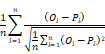
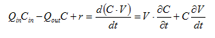
The volume of fluid in the tank depends on the net influent - effluent flow. If this is a negative value, then the volume of the tank will decrease until it reaches zero. At this point the effluent will equal the influent, regardless of the pump flow set. If the net influent-effluent flow is positive, the tank volume will increase until the maximum (specified by the user). At this point, the tank begins to overflow, so that the effluent flow (sum of the overflow and pump flows) will be equal to the influent flow. The effluent flow over and above the effluent pumped flow rates will leave through the overflow connection point. If the net influent-effluent flow is zero, then the volume will not change.
The mass balance for variable volume tanks is shown in Equations 2.1-2.4:
Equation 2.1
Equation 2.2
![]()
Equation 2.3
![]()
Equation 2.4

where:
Qin = influent flow rate (m3/d)
Qout = effluent flow rate (m3/d)
Cin = influent concentration (mg/L)
C = effluent concentration (mg/L)
r = rate of reaction (mg/L/d)
V = liquid volume (m3)
t = time (d)
Another feature of the objects with volume is their initial volume.
When a simulation begins, the user can specify what volume the tank
initially has through the use of a logical variable called
start with full tank, located under
Initial Conditions > Initial volume. If this
logical switch is true, then the tank will be full at the beginning
of the simulation.
If this logical variable is false, then the user can specify the initial reactor volumeat the start of the simulation. As a consequence of this, the user can specify the starting volume as full by two ways:
1. Either setting the logical variable as “true”; or
2. By setting the variable as “false” and manually specifying the starting volume as equal to the maximum tank volume.
From Equation 2.1, the concentration of a conservative material in objects with volume relative to its influent concentration can be calculated as shown in the following equations:
Equation 2.5
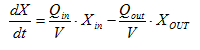
where:
X = conservative
component concentration (g/m3)
Q = flow rate
(m3/d)
t =
time (d)
Qin = influent
stream
Qout = effluent stream
Xout = effluent
concentration (g/m3)
At steady-state, the time derivatives are zero and Equation 2.5 becomes:
Equation 2.6
![]()
If the SRT is defined as:
Equation 2.7
![]()
where:
SRT = solids retention time (d)
V = volume
(m3)
Combining Equation 2.6 & Equation 2.7 gives:
Equation 2.8
![]()
The hydraulic residence time (HRT) is defined as:
Equation 2.9
![]()
Combining Equation 2.8 & Equation 2.9 gives:
Equation 2.10
![]()
This equation shows the ration of the concentration of the conservative component in the object to its concentration in the influent. At steady-state, it is directly proportional to the SRT/HRT value.
A library in GPS-X is a collection of wastewater process models using a set of basic wastewater components, or state variables. The term state variable refers to the basic variables that are continuously integrated over time. The composite variables are those variables that are calculated from (or composed of) the state variables. In discussing the state variables for the different libraries listed below, volume is not explicitly explained as a state variable as it is common to all libraries. The relationships presented in this chapter between the state and composite variables are used in every connection point of the plant layout.
NOTE: In GPS-X, BOD refers to the carbonaceous BOD5 (CBOD) unless otherwise stated. This is to distinguish the oxygen demand for organic carbon removal from the oxygen demand for ammonia oxidation. The values of these two analyses for the same sample can be considerably different.
Nine libraries are available for GPS-X:
· Comprehensive – Carbon, Nitrogen, Phosphorus, pH (MANTIS2LIB)
· Selenium and Sulfur (MANTIS2SLIB)
· Carbon Footprint – Carbon, Nitrogen, Phosphorus, pH (MANTIS3LIB)
· Process Water Treatment Library (PROCWATERLIB)
· Petrochemical Wastewater LIBRARY (MANTISIWLIB
· Carbon – Nitrogen (CNLIB)
· Carbon – Nitrogen – Industrial Pollutant (CNIPLIB)
· Carbon – Nitrogen – Phosphorus (CNPLIB)
· Carbon – Nitrogen – Phosphorus – Industrial Pollutant (CNPIPLIB)
NOTE: MANTIS3LIB is available to those who have purchased the Carbon Footprint Library add-on for their GPS-X license.
Fifty-two (52) state variables are available in the Comprehensive Model (MANTIS2LIB) library. (Table 3‑1)
Table 3‑1 - Comprehensie Model (MANTIS2LIB) Library State Variables
|
|
State Variables |
GPS-X Cryptic Symbols |
Units |
|
1. |
Dissolved oxygen |
so |
gO2/m3 |
|
2. |
Soluble inert organic |
si |
gCOD/m3 |
|
3. |
Colloidal organic substrate |
scol |
gCOD/m3 |
|
4. |
Fermentable substrate |
ss |
gCOD/m3 |
|
5. |
Acetate |
sac |
gCOD/m3 |
|
6. |
Propionate |
spro |
gCOD/m3 |
|
7. |
Methanol |
smet |
gCOD/m3 |
|
8. |
Dissolved hydrogen |
sh2 |
gCOD/m3 |
|
9. |
Dissolved methane |
sch4 |
gCOD/m3 |
|
10. |
Dissolved inorganic carbon |
stic |
gC/m3 |
|
11. |
Soluble organic nitrogen |
snd |
gN/m3 |
|
12. |
Ammonia nitrogen |
snh |
gN/m3 |
|
13. |
Nitrite nitrogen |
snoi |
gN/m3 |
|
14. |
Nitrate nitrogen |
snoa |
gN/m3 |
|
15. |
Dissolved nitrogen |
sn2 |
gN/m3 |
|
16. |
Ortho-phosphate |
sp |
gP/m3 |
|
17. |
Dissolved calcium |
sca |
gCa/m3 |
|
18. |
Dissolved magnesium |
smg |
gMg/m3 |
|
19. |
Dissolved potassium |
spot |
gK/m3 |
|
20. |
Dissolved cation |
scat |
eq/m3 |
|
21. |
Dissolved anion |
sana |
eq/m3 |
|
22. |
Inert Particulate |
xi |
gCOD/m3 |
|
23. |
Un-biodegradable cell decay material |
xu |
gO2/m3 |
|
24. |
Slowly biodegradable organics |
xs |
gCOD/m3 |
|
25. |
PHA accumulated in PAO |
xbt |
gCOD/m3 |
|
26. |
Heterotrophic biomass |
xbh |
gCOD/m3 |
|
27. |
Phosphate accumulating biomass |
xbp |
gCOD/m3 |
|
28. |
Ammonia oxidizer |
xbai |
gCOD/m3 |
|
29. |
Nitrite oxidizer |
xbaa |
gCOD/m3 |
|
30. |
Anammox biomass |
xbax |
gCOD/m3 |
|
31. |
Methylotrophic biomass |
xmet |
gCOD/m3 |
|
32. |
Fermentative biomass |
xbf |
gC/m3 |
|
33. |
Acetogen |
xbpro |
gN/m3 |
|
34. |
Acetate methanogens |
xbacm |
gN/m3 |
|
35. |
Hydrogen methanogens |
xbh2m |
gN/m3 |
|
36. |
Nitrogen in slowly deg. organics |
xns |
gN/m3 |
|
37. |
Phosphorous in slowly deg. organics |
xps |
gN/m3 |
|
38. |
Poly-phosphate accumulated in PAO |
xpp |
gP/m3 |
|
39. |
Particulate inert inorganic |
xii |
gCa/m3 |
|
40. |
Aluminum hydroxide |
xaloh |
gMg/m3 |
|
41. |
Aluminum phosphate |
xalpo4 |
gK/m3 |
|
42. |
Iron hydroxide |
xfeoh |
eq/m3 |
|
43. |
Iron phosphate |
xfepo4 |
eq/m3 |
|
44. |
Calcium carbonate |
xcaco3 |
gCOD/m3 |
|
45. |
Calcium phosphate |
xcapo4 |
gO2/m3 |
|
46. |
Magnesium hydrogen phosphate |
xmghpo4 |
gCOD/m3 |
|
47. |
Magnesium carbonate |
xmgco3 |
gCOD/m3 |
|
48. |
Ammonium magnesium phosphate(struvite) |
xmgnh4po4 |
gCOD/m3 |
|
49. |
Soluble component "a" |
sza |
gCOD/m3 |
|
50. |
Soluble component "b" |
szb |
gCOD/m3 |
|
51. |
Particulate component "a" |
xza |
gCOD/m3 |
|
52. |
Particulate component "b" |
xzb |
gCOD/m3 |
Seventy-two (72) state variables are available in the Sulphur and Selenium (MANTIS2SLIB) library. (Table 3‑2)
Table 3‑2 - Comprehensive Model (MANTIS2SLIB) Library State Variables
|
|
State Variables |
GPS-X Cryptic Symbols |
Units |
|
1. |
dissolved oxygen |
so |
gO2/m3 |
|
2. |
dissolved hydrogen gas |
sh2 |
gCOD/m3 |
|
3. |
dissolved dinitrogen gas |
sn2 |
gN/m3 |
|
4. |
dissolved methane |
sch4 |
gCOD/m3 |
|
5. |
readily degradable soluble substrate |
ss |
gCOD/m3 |
|
6. |
acetate |
sac |
gCOD/m3 |
|
7. |
propionate |
spro |
gCOD/m3 |
|
8. |
methanol |
smet |
gCOD/m3 |
|
9. |
colloidal substrate |
scol |
gCOD/m3 |
|
10. |
soluble inert material |
si |
gCOD/m3 |
|
11. |
slowly biodegradable substrate 1 |
xs1 |
gCOD/m3 |
|
12. |
slowly biodegradable substrate 2 |
xs2 |
gCOD/m3 |
|
13. |
slowly biodegradable substrate 3 |
xs3 |
gCOD/m3 |
|
14. |
poly-hydroxy alkanoates in PAO |
xbt |
gCOD/m3 |
|
15. |
unbiodegradable cell products |
xu |
gCOD/m3 |
|
16. |
particulate inert material |
xi |
gCOD/m3 |
|
17. |
ammonia nitrogen |
snh |
gN/m3 |
|
18. |
nitrite |
snoi |
gN/m3 |
|
19. |
nitrate |
snoa |
gN/m3 |
|
20. |
soluble organic nitrogen |
snd |
gN/m3 |
|
21. |
nitrogen in slowly biodegradable substrate |
xns |
gN/m3 |
|
22. |
selenate selenium |
sselna |
gSe/m3 |
|
23. |
selenite selenium |
sselni |
gSe/m3 |
|
24. |
elemental selenium |
xse0 |
gSe/m3 |
|
25. |
soluble sulfide sulfur |
stssul |
gS/m3 |
|
26. |
sulfate sulfur |
sso4 |
gS/m3 |
|
27. |
sulfite sulfur |
sso3 |
gS/m3 |
|
28. |
elemental sulfur |
xsul0 |
gS/m3 |
|
29. |
particulate heavy metal sulfide |
xhmes |
gS/m3 |
|
30. |
ortho-phosphate |
sp |
gP/m3 |
|
31. |
phosphorus in slowly biodegradable substrate |
xps |
gP/m3 |
|
32. |
poly-phosphate in PAO |
xpp |
gP/m3 |
|
33. |
heterotrophic biomass |
xbh |
gCOD/m3 |
|
34. |
ammonia oxidizer biomass |
xbai |
gCOD/m3 |
|
35. |
nitrite oxidixer biomass |
xbaa |
gCOD/m3 |
|
36. |
phosphate accumulating biomass |
xbp |
gCOD/m3 |
|
37. |
selenium-reducing biomass |
xbsel |
gCOD/m3 |
|
38. |
methylotrophic selenium-reducing biomass |
xbsemet |
gCOD/m3 |
|
39. |
propionate degrading sulfate-reducing biomass |
xbsr1 |
gCOD/m3 |
|
40. |
hydrogen utilizing sulfate-reducing biomass |
xbsr2 |
gCOD/m3 |
|
41. |
acetate utilizing sulfate-reducing biomass |
xbsr3 |
gCOD/m3 |
|
42. |
methanol utilizing sulfate-reducing biomass |
xbsr4 |
gCOD/m3 |
|
43. |
sulfur-oxiding biomass |
xbsox |
gCOD/m3 |
|
44. |
fermenting biomass |
xbf |
gCOD/m3 |
|
45. |
acetogenic biomass |
xbpro |
gCOD/m3 |
|
46. |
acetoclastic methanogenic biomass |
xbacm |
gCOD/m3 |
|
47. |
hydrogenotrophic methanogenic biomass |
xbh2m |
gCOD/m3 |
|
48. |
methylotrophic biomass |
xbmet |
gCOD/m3 |
|
49. |
methylotrophic methanogenic biomass |
xbmem |
gCOD/m3 |
|
50. |
anammox biomass |
xbax |
gCOD/m3 |
|
51. |
total soluble inorganic carbon |
stic |
gC/m3 |
|
52. |
total soluble calcium |
sca |
gCa/m3 |
|
53. |
soluble heavy metal |
shme |
gMe/m3 |
|
54. |
total soluble magnesium |
smg |
gMg/m3 |
|
55. |
total soluble potassium |
spot |
gK/m3 |
|
56. |
other cation |
scat |
eq/m3 |
|
57. |
other anion |
sana |
eq/m3 |
|
58. |
inorganic inert particulate |
xii |
gSS/m3 |
|
59. |
aluminum hydroxide |
xaloh |
gAl(OH)3/m3 |
|
60. |
aluminum phosphate |
xalpo4 |
gAlPO4/m3 |
|
61. |
iron hydroxide |
xfeoh |
gFe(OH)3/m3 |
|
62. |
iron sulfide |
xfes |
gFe(OH)3/m3 |
|
63. |
iron phosphate |
xfepo4 |
gFePO4/m3 |
|
64. |
calcium carbonate |
xcaco3 |
gCaCO3/m3 |
|
65. |
calcium phosphate |
xcapo4 |
gCaPO4/m3 |
|
66. |
magnesium carbonate |
xmgco3 |
gMgCO3/m3 |
|
67. |
magnesium hydrogen phosphate (newberyite) |
xmghpo4 |
gMgHPO4.3H2O/m3 |
|
68. |
magnesium ammonium phosphate (struvite) |
xmgnh4po4 |
gMgNH4PO4.6H2O/m3 |
|
69. |
soluble component a |
sza |
notset |
|
70. |
soluble component b |
szb |
notset |
|
71. |
particulate component a |
xza |
notset |
|
72. |
particulate component b |
xzb |
notset |
Fifty-six (56) state variables are available in the Carbon Footprint (MANTIS3LIB) Library. (Table 3‑3).
Table 3‑3 - Carbon Footprint (MANTIS3LIB) Library State Variables
|
|
State Variables |
GPS-X Cryptic Symbols |
Units |
|
1. |
Dissolved oxygen |
so |
gO2/m3 |
|
2. |
Soluble inert organic |
si |
gCOD/m3 |
|
3. |
Colloidal organic substrate |
scol |
gCOD/m3 |
|
4. |
Fermentable substrate |
ss |
gCOD/m3 |
|
5. |
Acetate |
sac |
gCOD/m3 |
|
6. |
Propionate |
spro |
gCOD/m3 |
|
7. |
Methanol |
smet |
gCOD/m3 |
|
8. |
Dissolved hydrogen |
sh2 |
gCOD/m3 |
|
9. |
Dissolved methane |
sch4 |
gCOD/m3 |
|
10. |
Dissolved inorganic carbon |
stic |
gC/m3 |
|
11. |
Soluble organic nitrogen |
snd |
gN/m3 |
|
12. |
Ammonia nitrogen |
snh |
gN/m3 |
|
13. |
Nitrite nitrogen |
snoi |
gN/m3 |
|
14. |
Nitrate nitrogen |
snoa |
gN/m3 |
|
15. |
Dissolved nitrogen |
sn2 |
gN/m3 |
|
16. |
Nitric oxide-Nitrogen |
snrio |
gN/m3 |
|
17. |
Nitrous Oxide |
snroo |
gN/m3 |
|
18. |
Hydroxylamine |
snh2oh |
gN/m3 |
|
19. |
Nitrosyl radical |
snoh |
gN/m3 |
|
20. |
Ortho-phosphate |
sp |
gP/m3 |
|
21. |
Dissolved calcium |
sca |
gCa/m3 |
|
22. |
Dissolved magnesium |
smg |
gMg/m3 |
|
23. |
Dissolved potassium |
spot |
gK/m3 |
|
24. |
Dissolved cation |
scat |
eq/m3 |
|
25. |
Dissolved anion |
sana |
eq/m3 |
|
26. |
Inert Particulate |
xi |
gCOD/m3 |
|
27. |
Un-biodegradable cell decay material |
xu |
gCOD/m3 |
|
28. |
Slowly biodegradable organics |
xs |
gCOD/m3 |
|
29. |
PHA accumulated in PAO |
xbt |
gCOD/m3 |
|
30. |
Heterotrophic biomass |
xbh |
gCOD/m3 |
|
31. |
Phosphate accumulating biomass |
xbp |
gCOD/m3 |
|
32. |
Ammonia oxidizer |
xbai |
gCOD/m3 |
|
33. |
Nitrite oxidizer |
xbaa |
gCOD/m3 |
|
34. |
Anammox biomass |
xbax |
g COD/m3 |
|
35. |
Methylotrophic biomass |
xmet |
g COD/m3 |
|
36. |
Fermentative biomass |
xbf |
g COD/m3 |
|
37. |
Acetogen |
xbpro |
gCOD/m3 |
|
38. |
Acetate methanogens |
xbacm |
gCOD/m3 |
|
39. |
Hydrogen methanogens |
xbh2m |
gCOD/m3 |
|
40. |
Nitrogen in slowly deg. organics |
xns |
gN/m3 |
|
41. |
Phosphorous in slowly deg. organics |
xps |
gP/m3 |
|
42. |
Poly-phosphate accumulated in PAO |
xpp |
gP/m3 |
|
43. |
Particulate inert inorganic |
xii |
g/m3 |
|
44. |
Aluminum hydroxide |
xaloh |
gAl(OH)3/m3 |
|
45. |
Aluminum phosphate |
xalpo4 |
gAlPO4/m3 |
|
46. |
Iron hydroxide |
xfeoh |
gFe(OH)3/m3 |
|
47. |
Iron phosphate |
xfepo4 |
gFePO4/m3 |
|
48. |
Calcium carbonate |
xcaco3 |
gCaCO3/m3 |
|
49. |
Calcium phosphate |
xcapo4 |
gCa3(PO4)2/m3 |
|
50. |
Magnesium hydrogen phosphate |
xmghpo4 |
gMgHPO4.3H2O/m3 |
|
51. |
Magnesium carbonate |
xmgco3 |
gMgCO3/m3 |
|
52. |
Ammonium magnesium phosphate(struvite) |
xmgnh4po4 |
gMgNH4PO4.6H2O /m3 |
|
53. |
Soluble component "a" |
sza |
notset |
|
54. |
Soluble component "b" |
szb |
notset |
|
55. |
Particulate component "a" |
xza |
notset |
|
56. |
Particulate component "b" |
xzb |
notset |
Sixteen state variables are available in the Carbon – Nitrogen library (Table 3‑4)
Table 3‑4 – Carbon – Nitrogen Library (CNLIB) State Variables
|
|
State Variables |
GPS-X Cryptic Symbols |
Units |
|
1. |
Soluble inert organics |
si |
gCOD/m3 |
|
2. |
Readily biodegradable (soluble) substrate |
ss |
gCOD/m3 |
|
3. |
Particulate inert organics |
xi |
gCOD/m3 |
|
4. |
Slowly biodegr. (stored, particulate) substrate |
xs |
gCOD/m3 |
|
5. |
Active heterotrophic biomass |
xbh |
gCOD/m3 |
|
6. |
Active autotrophic biomass |
xba |
gCOD/m3 |
|
7. |
Unbiodegradable particulates from cell decay |
xu |
gCOD/m3 |
|
8. |
Cell internal storage product |
xsto |
gCOD/m3 |
|
9. |
Dissolved oxygen |
so |
gN/m3 |
|
10. |
Nitrate and nitrite N |
sno |
gN/m3 |
|
11. |
Free and ionized ammonia |
snh |
gN/m3 |
|
12. |
Soluble biodegradable organic nitrogen (in ss) |
snd |
gN/m3 |
|
13. |
Particulate biodegr. organic nitrogen (in xs) |
xnd |
gN/m3 |
|
14. |
Dinitrogen |
snn |
gN/m3 |
|
15. |
Alkalinity |
salk |
mole/m3 |
|
16. |
Inert inorganic suspended solids |
xii |
g/m3 |
Forty-six (46) state variables are available in the Industrial Pollutant library. Sixteen (16) are pre-defined and thirty (30) are user-definable (15 soluble, 15 particulate). They are listed in Table 3‑5.
Table 3‑5 – Industrial Pollutant (CNIPLIB) Library State Variables
|
|
State Variables |
GPS-X Cryptic Symbols |
Units |
|
1. |
Soluble inert organics |
si |
gCOD/m3 |
|
2. |
Readily biodegradable (soluble) substrate |
ss |
gCOD/m3 |
|
3. |
Particulate inert organics |
xi |
gCOD/m3 |
|
4. |
Slowly biodegr. (stored, particulate) substrate |
xs |
gCOD/m3 |
|
5. |
Active heterotrophic biomass |
xbh |
gCOD/m3 |
|
6. |
Active autotrophic biomass |
xba |
gCOD/m3 |
|
7. |
Unbiodegradable particulates from cell decay |
xu |
gCOD/m3 |
|
8. |
Cell internal storage product |
xsto |
gCOD/m3 |
|
9. |
Dissolved oxygen |
so |
gO2/m3 |
|
10. |
Nitrate and nitrite N |
sno |
gN/m3 |
|
11. |
Free and ionized ammonia |
snh |
gN/m3 |
|
12. |
Soluble biodegradable organic nitrogen (in ss) |
snd |
gN/m3 |
|
13. |
Particulate biodegradable organic nitrogen (in xs) |
xnd |
gN/m3 |
|
14. |
Dinitrogen |
snn |
gN/m3 |
|
15. |
Alkalinity |
salk |
mole/m3 |
|
16. |
Inert inorganic suspended solids |
xii |
g/m3 |
|
17. |
Soluble component "a" |
sza |
notset |
|
18. |
Soluble component "b" |
szb |
notset |
|
19. |
Soluble component "c" |
szc |
notset |
|
20. |
Soluble component "d" |
szd |
notset |
|
21. |
Soluble component "e" |
sze |
notset |
|
22. |
Soluble component "f" |
szf |
notset |
|
23. |
Soluble component "g" |
szg |
notset |
|
24. |
Soluble component "h" |
szh |
notset |
|
25. |
Soluble component "i" |
szi |
notset |
|
26. |
Soluble component "j" |
szj |
notset |
|
27. |
Soluble component "k" |
szk |
notset |
|
28. |
Soluble component "l" |
szl |
notset |
|
29. |
Soluble component "m" |
szm |
notset |
|
30. |
Soluble component "n" |
szn |
notset |
|
31. |
Soluble component "o" |
szo |
notset |
|
32. |
Particulate component "a" |
xza |
notset |
|
33. |
Particulate component "b" |
xzb |
notset |
|
34. |
Particulate component "c" |
xzc |
notset |
|
35. |
Particulate component "d" |
xzd |
notset |
|
36. |
Particulate component "e" |
xze |
notset |
|
37. |
Particulate component "f" |
xzf |
notset |
|
38. |
Particulate component "g" |
xzg |
notset |
|
39. |
Particulate component "h" |
xzh |
notset |
|
40. |
Particulate component "i" |
xzi |
notset |
|
41. |
Particulate component "j" |
xzj |
notset |
|
42. |
Particulate component "k" |
xzk |
notset |
|
43. |
Particulate component "l" |
xzl |
notset |
|
44. |
Particulate component "m" |
xzm |
notset |
|
45. |
Particulate component "n" |
xzn |
notset |
|
46. |
Particulate component "o" |
xzo |
notset |
Twenty-seven (27) state variables are available in the Carbon – Nitrogen – Phosphorus library (Table 3‑6)
Table 3‑6 – Carbon – Nitrogen – Phosphorus (CNPLIB) Library State Variables
|
|
State Variables |
GPS-X Cryptic Symbols |
Units |
|
1. |
Soluble inert organics |
si |
gCOD/m3 |
|
2. |
Readily biodegradable (soluble) substrate |
ss |
gCOD/m3 |
|
3. |
Particulate inert organics |
xi |
gCOD/m3 |
|
4. |
Slowly biodegr. (stored, particulate) substrate |
xs |
gCOD/m3 |
|
5. |
Active heterotrophic biomass |
xbh |
gCOD/m3 |
|
6. |
Active autotrophic biomass |
xba |
gCOD/m3 |
|
7. |
Unbiodegradable particulates from cell decay |
xu |
gCOD/m3 |
|
8. |
Dissolved oxygen |
so |
gO2/m3 |
|
9. |
Nitrate and nitrite N |
sno |
gN/m3 |
|
10. |
Free and ionized ammonia |
snh |
gN/m3 |
|
11. |
Soluble biodegradable organic nitrogen (in ss) |
snd |
gN/m3 |
|
12. |
Particulate biodegradable organic nitrogen (in xs) |
xnd |
gN/m3 |
|
13. |
Polyphosphate accumulating biomass |
xbp |
gCOD/m3 |
|
14. |
Poly-hydroxy-alkanoates (PHA) |
xbt |
gCOD/m3 |
|
15. |
Stored polyphosphate |
xpp |
gP/m3 |
|
16. |
Volatile fatty acids |
slf |
gCOD/m3 |
|
17. |
Soluble phosphorus |
sp |
gP/m3 |
|
18. |
Alkalinity |
salk |
mole/m3 |
|
19. |
Dinitrogen |
snn |
gN/m3 |
|
20. |
Soluble unbiodegradable organic nitrogen (in si) |
sni |
gN/m3 |
|
21. |
Fermentable readily biodegradable substrate |
sf |
gCOD/m3 |
|
22. |
Stored glycogen |
xgly |
gCOD/m3 |
|
23. |
Stored polyphosphate (releasable) |
xppr |
gP/m3 |
|
24. |
Metal-hydroxides |
xmeoh |
g/m3 |
|
25. |
Metal-phosphate |
xmep |
g/m3 |
|
26. |
Cell internal storage product |
xsto |
gCOD/m3 |
|
27. |
Inert inorganic suspended solids |
xii |
g/m3 |
Fifty-seven (57) state variables are available in the CNP Industrial Pollutant Library (CNPIPLIB). These include the 27 state variables from CNPLIB, as well as 30 user‑definable variables (15 soluble and 15 particulate) as shown in Table 3‑7
Table 3‑7 – CNP Industrial Pollutant (CNPIPLIB) Library State Variables
|
|
State Variables |
GPS-X Cryptic Symbols |
Units |
|
1. |
Soluble inert organics |
si |
gCOD/m3 |
|
2. |
Readily biodegradable (soluble) substrate |
ss |
gCOD/m3 |
|
3. |
Particulate inert organics |
xi |
gCOD/m3 |
|
4. |
Slowly biodegr. (stored, particulate) substrate |
xs |
gCOD/m3 |
|
5. |
Active heterotrophic biomass |
xbh |
gCOD/m3 |
|
6. |
Active autotrophic biomass |
xba |
gCOD/m3 |
|
7. |
Unbiodegradable particulates from cell decay |
xu |
gCOD/m3 |
|
8. |
Dissolved oxygen |
so |
gO2/m3 |
|
9. |
Nitrate and nitrite N |
sno |
gN/m3 |
|
10. |
Free and ionized ammonia |
snh |
gN/m3 |
|
11. |
Soluble biodegradable organic nitrogen (in ss) |
snd |
gN/m3 |
|
12. |
Particulate biodegradable organic nitrogen (in xs) |
xnd |
gN/m3 |
|
13. |
Polyphosphate accumulating biomass |
xbp |
gCOD/m3 |
|
14. |
Poly-hydroxy-alkanoates (PHA) |
xbt |
gCOD/m3 |
|
15. |
Stored polyphosphate |
xpp |
gP/m3 |
|
16. |
Volatile fatty acids |
slf |
gCOD/m3 |
|
17. |
Soluble phosphorus |
sp |
gP/m3 |
|
18. |
Alkalinity |
salk |
mole/m3 |
|
19. |
Dinitrogen |
snn |
gN/m3 |
|
20. |
Soluble unbiodegradable organic nitrogen (in si) |
sni |
gN/m3 |
|
21. |
Fermentable readily biodegradable substrate |
sf |
gCOD/m3 |
|
22. |
Stored glycogen |
xgly |
gCOD/m3 |
|
23. |
Stored polyphosphate (releasable) |
xppr |
gP/m3 |
|
24. |
Metal-hydroxides |
xmeoh |
g/m3 |
|
25. |
Metal-phosphate |
xmep |
g/m3 |
|
26. |
Cell internal storage product |
xsto |
gCOD/m3 |
|
27. |
Inert inorganic suspended solids |
xii |
g/m3 |
|
28. |
Soluble component "a" |
sza |
notset |
|
29. |
Soluble component "b" |
szb |
notset |
|
30. |
Soluble component "c" |
szc |
notset |
|
31. |
Soluble component "d" |
szd |
notset |
|
32. |
Soluble component "e" |
sze |
notset |
|
33. |
Soluble component "f" |
szf |
notset |
|
34. |
Soluble component "g" |
szg |
notset |
|
35. |
Soluble component "h" |
szh |
notset |
|
36. |
Soluble component "i" |
szi |
notset |
|
37. |
Soluble component "j" |
szj |
notset |
|
38. |
Soluble component "k" |
szk |
notset |
|
39. |
Soluble component "l" |
szl |
notset |
|
40. |
Soluble component "m" |
szm |
notset |
|
41. |
Soluble component "n" |
||
|
42. |
Soluble component "o" |
||
|
43. |
Particulate component "a" |
||
|
44. |
Particulate component "b" |
||
|
45. |
Particulate component "c" |
||
|
46. |
Particulate component "d" |
||
|
47. |
Particulate component "e" |
||
|
48. |
Particulate component "f" |
||
|
49. |
Particulate component "g" |
||
|
50. |
Particulate component "h" |
||
|
51. |
Particulate component "i" |
||
|
52. |
Particulate component "j" |
||
|
53. |
Particulate component "k" |
||
|
54. |
Particulate component "l" |
||
|
55. |
Particulate component "m" |
||
|
56. |
Particulate component "n" |
||
|
57. |
Particulate component "o" |
In GPS-X, a group of state variables (such as oxygen, heterotrophic biomass, nitrate, ammonia, soluble substrate, particulate substrate, etc.) are calculated for each connection point in the plant layout. These state variables are the fundamental components that are acted upon by the processes in the models in each library.
These particular state variable components are not always easily measurable or interpretable in practical applications. Therefore, a series of composite variables are calculated from the state variables. The composite variables combine the state variables into forms that are typically measured, such as total suspended solids (TSS), BOD, COD and Total Kjeldahl Nitrogen (TKN).
The way that the composite variables are calculated from state variables changes from library to library and to a great degree from model to model.
Composite variables are calculated from state variables with the use of stoichiometric constants. These constants describe the relationships between various states and composites, and depend on the type of composite calculations used.
In this chapter, diagrams and tables are used to depict the relationships between the state and composite variables included in a library.
The nomenclature used in the box-and-arrows diagrams is explained in Figure 4‑1.
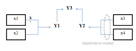
Figure 4‑1 – Diagram Nomenclature
The variables in the boxes and above the connection lines are known (either previously calculated or user input). The variables in BOLD CAPITALS represent the composite variables which are to be calculated. The connection line shows the direction of calculation and always begins from a known or boxed variable. Multiple lines converging to one unknown variable imply a summation operator. In the example shown above, the variable Y1 is calculated by multiplying the variable x1 by the stoichiometry parameter k and summing it with variable x2. If no stoichiometry parameter appears above the connection line, it implies a default value of 1. When a broken line circle is drawn on the lines, it indicates that the stoichiometry parameters for these lines are model dependent. In certain situations two or more calculated composite variables are used to calculate an additional composite variable. For example, Y3 is calculated by adding the calculated composite variables of Y1 and Y2.
In addition to diagrams which explain the general way composite variables are calculated, composite variable tables are used to explain model-specific calculations. The nomenclature used in the composite variables tables is explained in Table 4‑1:
Table 4‑1 – Example Composite Variable Calculations
|
|
SCOMP |
XCOMP |
TCOMP |
|
sa |
1 |
|
1 |
|
sb |
ksb |
|
ksb |
|
xa |
|
1 |
1 |
|
xb |
|
kxb |
kxb |
The composite variables being calculated are shown across the top of each column. The state variables used in the calculations are shown down the left side of the table. To calculate the composite variable, each state variable is multiplied by the coefficient in the table for that particular composite variable, and then summed down the column.
For the example data given in Table 4‑1, the calculations for SCOMP, XCOMP, and TCOMP are:
SCOMP = 1*sa + ksb*sb + 0*xa + 0*xb = sa + ksb*sb
XCOMP = 0*sa + 0*sb + 1*xa + kxb*xb = xa + kxb*xb
TCOMP = 1*sa + ksb*sb + 1*xa + kxb*xb = sa + ksb*sb +
xa + kxb*xb
Figure 4‑2 shows the relationship between the CNLIB state variables and the TSS, BOD, and COD composite state variables. Table 4‑2 illustrates the same composite variable calculations in the tabular format.
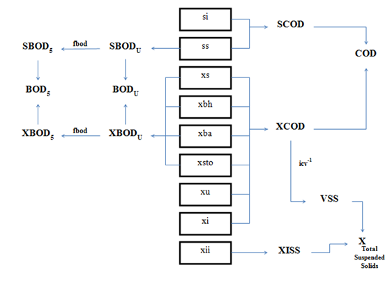
Figure 4‑2 – Carbon – Nitrogen Library (CNLIB): BOD, COD, and Suspended Solids Composite Variables and their Relationship to the State Variables
Table 4‑2 – CNLIB BOD, COD, and TSS Composite Variables (All Models)
|
|
||||||||||||
The COD composite variables are a sum of state variables (where units are gCOD/m3). Soluble COD (SCOD) is the sum of the soluble inert organics (si) and readily biodegradable substrate (ss), while particulate COD (XCOD) is the sum of the slowly biodegradable substrate (xs), active heterotrophic biomass (xbh), active autotrophic biomass (xba), cell internal storage product (xsto), un-biodegradable particulates from cell decay (xu), and particulate inert organics (xi). The total COD (COD) is the sum of the soluble and particulate COD.
The suspended solids composite variable (X) is calculated from the particulate COD (XCOD) by dividing it by the XCOD: VSS ratio (icv), which changes the units of the XCOD to mgVSS/L, resulting in the volatile suspended solids (VSS) composite variable. To calculate the suspended solids composite variable (X), VSS is added to particulate inert inorganic material (XII). By default in the CN library, particulate inert suspended solids (XISS) is equal to xii.
The biochemical oxygen demand (BOD) composite variables are calculated from the state variables. First, the biodegradable state variables (the state variables that exert BOD, which are in units of gO/m3) are summed to provide both a particulate and a soluble ultimate BOD (XBODU, SBODU). The sum of these components is the total ultimate BOD measurement (BODU). To determine BOD5, the calculated BODU is multiplied by a stoichiometric fraction, fbod, which is the ratio of BOD5:BODU.
In terms of variables containing nitrogen, the
calculation of the composite variables involves adding up various
state variables and multiplying other state variables by fractions
as appropriate (Figure
4‑3). The soluble total
Kjeldahl nitrogen (STKN) is the sum of the free and
ionized ammonia (snh), soluble biodegradable organic
nitrogen (snd), and (in asm3 only) the
nitrogen components of soluble substrate (ss) and soluble
inerts (si). The particulate total Kjeldahl nitrogen
(XTKN) is the particulate biodegradable organic
nitrogen (xnd), plus the nitrogen component of biomass
(xbh and xba), unbiodegradable cell products
(xu), particulate substrate (xs) and particulate
inerts (xi). Total Kjeldahl nitrogen (TKN) is
the sum of soluble (STKN) and particulate TKN
(XTKN). The total nitrogen (TN) is the
sum of the TKN and the nitrate nitrogen
(sno).
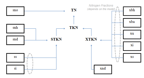
Figure 4‑3 – Carbon – Nitrogen Library: Composite Variables and their Relationships to the State Variables
The nitrogen fractions of xbh, xba, xu, xi, ss and si vary from model to model. The nitrogen composite variable relationships for the mantis, asm1 and asm3 models are shown in Table 4‑3, Table 4‑4, and Table 4‑5
Table 4‑3 – CNLIB Nitrogen Composite Variables – MANTIS Model
|
|
STKN |
|||
|
sno |
|
|||
|
snh |
1 |
|||
|
snd |
1 |
|||
|
xnd |
|
|||
|
xbh |
|
|||
|
xba |
|
|||
|
xu |
|
|||
|
xi |
|
Table 4‑4 – CNLIB Nitrogen Composite Variables – ASM1 Model
|
|
STKN |
XTKN |
TKN |
TN |
|
sno |
|
|||
|
snh |
1 |
|||
|
snd |
1 |
|||
|
xnd |
|
|||
|
xbh |
|
|||
|
xba |
|
|||
|
xu |
|
|||
|
xi |
|
Table 4‑5 - CNLIB Nitrogen Composite Variables - ASM3 Model
|
|
||||
The relationship between the state and composite variables are the same as those for CNLIB (Figure 4‑3 and Table 4‑5). Table 4‑3 through Table 4‑5 illustrates the composite variable calculations for the mantis1, asm1, and asm3 models in CNIPLIB.
Figure 4‑4 shows the relationships between CNPLIB state variables and the TSS, BOD and COD composite variables. Table 4‑6 illustrates the same composite variable calculations in tabular format.
As all the state
variables are in units of gCOD/m3, the COD composite
variables are simply a sum of the appropriate state variables. In
general, the soluble COD (SCOD) is a sum of the
soluble inert organics (si), volatile fatty acids
(slf), fermentable readily biodegradable substrate
(sf), and readily biodegradable substrate (ss). The
particulate COD (XCOD) is a sum of the slowly
biodegradable substrate (xs), active heterotrophic biomass
(xbh), active autotrophic biomass (xba),
polyphosphate accumulating biomass (xbp), stored glycogen
(xgly), poly-hydroxy-alkanoates (xbt),
unbiodegradable particulates from cell decay (xu), cell
internal storage product (xsto) and particulate inert
organics (xi). The total COD (COD) is the sum
of the soluble and particulate COD.
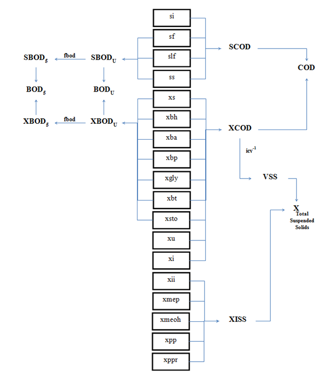
Figure 4‑4 – Carbon – Nitrogen – Phosphorus Library: BOD, COD, and Suspended Solids Composite Variables and their Relationship to the State Variables
The suspended solids composite variable is calculated from the particulate COD (XCOD) by dividing it by the XCOD:VSS ratio (icv). This changes the units of the XCOD to gVSS/m3, resulting in the composite variable for volatile suspended solids (VSS). To calculate the suspended solids composite variable (X), VSS is added to the concentration of inert inorganic particulates (XII), metal hydroxides (xmeoh) and metal phosphates (xmep), and stored polyphosphate (multiplied by 3 to change from gP/m3 to g/m3).
The biochemical oxygen demand (BOD) composite variables are calculated from the state variables. The biodegradable state variables (the state variables that exert BOD, which are in units of gCOD/m3) are summed to provide a particulate and a soluble ultimate BOD (XBODU, SBODU). The sum of these components is the total ultimate BOD measurement (BODU). To determine BOD5, a stoichiometric fraction, fbod, which is the ratio of BOD5:BOD20, is multiplied by the calculated BODU.
Table 4‑6 - CNPLIB BOD, COD, and TSS Composite Variables
|
|
SBODU |
XBODU |
BODU |
SBOD |
XBOD |
BOD |
SCOD |
XCOD |
COD |
VSS |
XISS |
X |
|
ss |
1 |
|
|
|
|
|
|
|||||
|
sf |
1 |
|
|
|
|
|
|
|||||
|
slf |
1 |
|
|
|
|
|
|
|||||
|
xs |
|
|
|
|
||||||||
|
xbh |
|
|
|
|
||||||||
|
xba |
|
|
|
|
||||||||
|
xpb |
|
|
|
|
||||||||
|
si |
|
|
|
|
|
|
|
|
|
|
||
|
xi |
|
|
|
|
|
|
|
|
||||
|
xu |
|
|
|
|
|
|
|
|
||||
|
xgly |
|
|
|
|
||||||||
|
xbt |
|
|
|
|
||||||||
|
xsto |
|
|
|
|
||||||||
|
xii |
|
|
|
|
|
|
|
|
|
|
||
|
xmeoh |
|
|
|
|
|
|
|
|
|
|
||
|
xmep |
|
|
|
|
|
|
|
|
|
|
||
|
xpp |
|
|
|
|
|
|
|
|
|
|
||
|
xppr |
|
|
|
|
|
|
|
|
|
|
In terms of variables containing nitrogen, the calculation of the
composite variables is similar to the calculations done in the
Carbon - Nitrogen library. The differences include the addition of
a new state variable, soluble unbiodegradable organic nitrogen
(sni), to the soluble TKN (STKN), the
inclusion of nitrogen components of the new substrate type
(sf), and the inclusion of nitrogen components of
poly‑phosphate-accumulating organisms (xbp). See
Figure 4‑5 for a general diagram of the nitrogen
composite variable calculations.
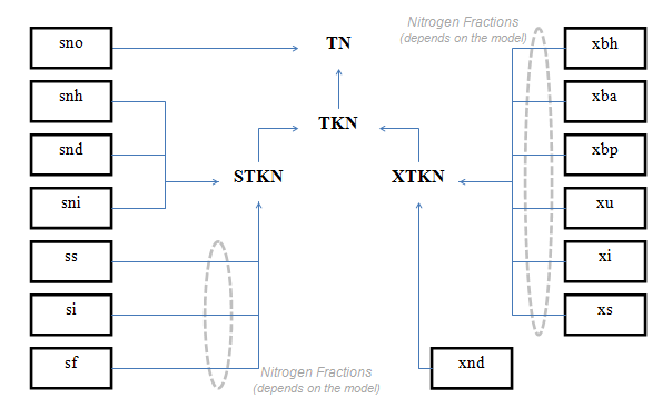
Figure 4‑5 - Carbon - Nitrogen - Phosphorus Library: Nitrogen Composite Variables and their Relationships to the State Variables
Table 4‑7 - CNPLIB Nitrogen Composite Variables - MANTIS Model
|
|
STKN |
|||
|
sno |
||||
|
snh |
||||
|
sni |
||||
|
snd |
||||
|
xnd |
||||
|
xbh |
||||
|
xba |
||||
|
xi |
||||
|
xu |
The calculation for nitrogen state variables differs slightly from model to model. In particular, the nitrogen fractions of biomass and other particulate components have different names from model to model. Table 4‑7 through Table 4‑11 shows the nitrogen composite variable calculations for the mantis, asm1, asm2d, asm3 and newgeneral models in CNPLIB.
Table 4‑8 - CNPLIB Nitrogen Composite Variables - ASM1 Model
|
|
||||
Table 4‑9 - CNPLIB Nitrogen Composite Variables - ASM2d Model
Table 4‑10 - CNPLIB Nitrogen Composite Variables - ASM3 Model
Table 4‑11 - CNPLIB Nitrogen Composite Variables - NEWGENERAL model
|
|
STKN |
XTKN |
TKN |
TN |
|
sno |
|
|
|
1 |
|
snh |
1 |
|
1 |
1 |
|
sni |
1 |
|
1 |
1 |
|
snd |
1 |
|
1 |
1 |
|
xnd |
|
1 |
1 |
1 |
|
xbp |
|
fnzh |
fnzh |
fnzh |
|
xbh |
|
fnzh |
fnzh |
fnzh |
|
xba |
|
fnzh |
fnzh |
fnzh |
|
xi |
|
fnzeh |
fnzeh |
fnzeh |
|
xu |
|
fnzeh |
fnzeh |
fnzeh |
Generally, soluble total phosphorus (STP) is equal to the sum of soluble phosphorus (sp) and the phosphorus components of ss, si, and sf, as appropriate. Particulate total phosphorus (XTP) is the sum of stored polyphosphate (xpp and xppr) and the phosphorus components of xs, xi, xbh, xba, xbp and xmeoh. See Figure 4‑6 for a schematic of these calculations. The calculations differ slightly from model to model. Table 4‑12 to
Table 4‑15 describe the
phosphorus composite variable calculations.
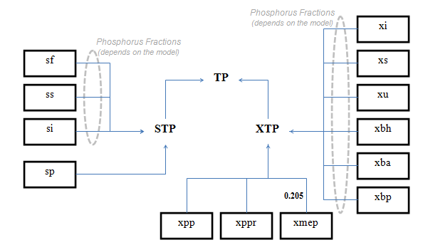
Figure 4‑6 - Carbon - Nitrogen - Phosphorus Library: Phosphorus Composite Variables and their Relationship to the State Variables
Table 4‑12 - CNPLIB Phosphorus Composite Variables - ASM1/MANTIS Models
Table 4‑13 – CNPLIB Phosphorus Composite Variables – ASM3 Model
|
|
STP |
XTP |
TP |
|
sp |
1 |
||
|
ss |
ipss |
||
|
si |
ipsi |
||
|
xi |
|
||
|
xs |
|
||
|
xbh |
|
||
|
xba |
|
||
|
xbp |
|
||
|
xmep |
|
||
|
xpp |
|
||
|
xppr |
|
Table 4‑14 - CNPLIB Phosphorus Composite Variables - ASM2d Model
|
|
STP |
XTP |
TP |
|
sp |
1 |
||
|
sf |
ipsf |
||
|
si |
ipsi |
||
|
xi |
|
||
|
xs |
|
||
|
xbh |
|
||
|
xba |
|
||
|
xbp |
|
||
|
xmep |
|
||
|
xpp |
|
||
|
xppr |
|
Table 4‑15 - CNPLIB Phosphorus Composite Variables - NEWGENERAL Model
|
|
STP |
XTP |
TP |
|
sp |
|||
|
xpp |
|||
|
xppr |
|||
|
xi |
|||
|
xu |
|||
|
xbh |
|||
|
xba |
|||
|
xbp |
|||
|
xmep |
The relationships between the state variables and composite variables are similar to the Carbon-Nitrogen-Phosphorus library (CNPLIB). Table 4‑7 through
Table 4‑15 shows the relationships between the state and composite variables that are used in the models in CNPIPLIB.
The composite variable calculation schemes in MANTSI2LIB are shown in Figure 4‑7 to Figure 4‑11. Figure 4‑7 shows the scheme for estimation of soluble BOD5 (SBOD), particulate BOD5 (XBOD), BOD5 (BOD), soluble ultimate BOD (SBODU), particulate ultimate BOD (SBODU), ultimate BOD (BODU), soluble COD (SCOD), particulate COD (XCOD) and COD (COD). The list of stoichiometric parameters used in the estimation of composite variables is provided in Table 4‑16.
Table 4‑16 - Stoichiometry Parameters used in Estimation of Composite Variables
|
Stoichiometry Parameter |
Default Value |
Description |
|
yhglobal |
0.666 |
Heterotrophic biomass yield |
|
fuu |
0.206 |
Fraction of unbiodegradable residue in biomass |
|
fssbodtosscod |
0.717 |
BOD5 to COD ratio of soluble substrate |
|
fpsbodtopscod |
0.58 |
BOD5 to COD ratio of particulate substrate |
|
fbbodtobcod |
0.566 |
BOD5 to COD ratio of biomass |
|
icodtovssxbt |
1.674 |
xCOD/VSS ratio of PHA |
The default value of the stoichiometry parameters can be changed in
the
System > Input Parameters > Global Fixed
stoichiometry menu.
Figure 4‑8 shows the scheme for estimation of
Volatile Suspended Solid (VSS), Inorganic Suspended Solid
(XISS) and Total Suspended Solid (TSS) concentration.
In the estimation of VSS, each biomass concentration is
multiplied by a corresponding VSS to COD factor. For
example, ivsstocodxbh is the VSS to COD
ratio for heterotrophic biomass, xbh. The VSS
to COD ratio for each biomass type are calculated based on
the biomass composition. The default composition of biomass can be
accessed and changed in the
System > Input Parameters > Global Fixed
stoichiometry menu.
As the composition of xs and xi are not well known,
the VSS to COD ratios for these states
ivsstocodxs and ivsstocodxi are
provided as direct inputs. These ratios can be accessed and changed
in System > Input Parameters > Influent
Stoichiometry menu. The state variable of xns is
included in the calculation of VSS for being consistent with
the practice of considering the N fraction in biomass as part of
VSS. A stoichiometry factor of 17.0/14.0 is used to convert
N to NH3.
In the calculation of Inorganic Suspended Solid (XISS), each biomass concentration is multiplied by the inorganic fraction in the biomass. The inorganic fraction for each biomass is estimated by subtracting the VSS to SS ratio for each individual biomass from one. The VSS to SS ratio for each individual biomass type is calculated by using the set biomass composition, for example ivsstossxbh is the VSS to SS ratio calculated for the xbh biomass type.
The composite variable of XISS also includes the contribution from the inorganic states in the model. The mass contributions from the xpp and xps states are calculated by using a stoichiometry factor of 95/31. The factor reflects the conversion from molecular weight of P to molecular weight of PO43-. For all the other inorganic states a stoichiometry ratio of 1 is used.
The Total Suspended Solid (TSS) concentration is calculated by the sum of estimated VSS and XISS.
Figure 4‑9 shows the scheme for estimation of soluble part of Total Kjeldahl Nitrogen (STKN), particulate part of Total Kjeldahl Nitrogen (XTKN), Total Kjeldahl Nitrogen (TKN), Total Nitrogen (TN) and Total Nitrogen including dissolved Nitrogen (TN & dissolved gas). In the estimation of STKN, the stoichiometry ratio of, insi is used to estimate the organic nitrogen present in the si state variable. In the estimation of XTKN, each biomass concentration is multiplied by a corresponding stoichiometry factor representing the N content in the corresponding biomass. For example, inxbh is the stoichiometry factor representing the N content in the heterotrophic biomass, xbh. The N fraction for each biomass type is calculated based on the biomass composition. The default composition of biomass can be accessed and changed in the System > Input Parameters > Global Fixed stoichiometry menu. In the calculation of XTKN, the N contained in the MgNH4PO4 is also included. Although, in strict sense this is not a part of the organic nitrogen, it is assumed that the ammonia contained in the precipitate shall reflect in the analytical measurement of TKN.
Figure
4‑10 shows the scheme for estimation of soluble part of
Total Phosphorus (STP), particulate organic part of Total
Phosphorus (XTOP), particulate inorganic part of Total
Phosphorus (XTIP) and Total Phosphorus. In the estimation of
STP, the stoichiometry ratio of, ipnsi is used to
estimate the phosphorus present in the si state
variable. In the estimation of XTOP, each biomass
concentration is multiplied by a corresponding stoichiometry factor
representing the P content in the corresponding biomass. For
example, ipxbh is the stoichiometry factor
representing the P content in the heterotrophic biomass,
xbh. The P fraction for each biomass type is
calculated based on the biomass composition. The default
composition of biomass can be accessed and changed in the
System > Input Parameters > Global Fixed
stoichiometry menu. In the calculation of XTIP, the
P contained in various P- precipitates is included. The
stoichiometry factor for each precipitate are estimated based on
the composition of the precipitate. These stoichiometry factors are
also available in Global Fixed stoichiometry menu. The
composite variable of XTP is estimated by the sum of
XTOP and XTIP. The TP is estimated by the sum of
STP and XTP.
Figure
4‑11 shows the scheme for estimation of soluble part of
Total Organic Carbon (STOC), particulate part of Total
Organic Carbon (XTOC), and Total Organic Carbon. In the
estimation of STOC, the stoichiometry ratio of icsac,
icsmet, icspro are estimated based on the substrate
compositions. The stoichiometry factor of icscol,
icsi and icss on the other hand needs to be set by
direct user input. These factors can be accessed and changed in
System > Input Parameters > Influent
stoichiometry menu. In the estimation of XTOC, each
biomass concentration is multiplied by a corresponding
stoichiometry factor representing the C content in the
corresponding biomass. For example, icpxbh is the
stoichiometry factor representing the C content in the
heterotrophic biomass, xbh. The C fraction for each
biomass type is calculated based on the biomass composition. The
default composition of biomass can be accessed and changed in the
System > Input Parameters > Global Fixed
stoichiometry menu. For the particulate states of xi
and xs, the user can directly enter the C content in the
System > Input Parameters > Influent
stoichiometry menu. The composite variable of TOC is
estimated by the sum of XTOC and STOC.
Table 4‑17 presents the summary of the stoichiometry parameters used in the MANTSI2LIB and access menus for changing the default values.
Table 4‑17 - Access Menus for Different Stoichiometry Parameters in MANTIS2LIB
|
Stoichiometry Parameter |
Access Menu |
|
yhglobal |
System > Input Parameters > Global Fixed stoichiometry |
|
fuu |
System > Input Parameters > Global Fixed stoichiometry |
|
fssbodtosscod |
System > Input Parameters > Global Fixed stoichiometry |
|
fpsbodtopscod |
System > Input Parameters > Global Fixed stoichiometry |
|
fbbodtobcod |
System > Input Parameters > Global Fixed stoichiometry |
|
COD to VSS ratio for biomass |
System > Input Parameters > Global Fixed stoichiometry (Calculated based on biomass composition) |
|
COD to VSS ratio for xs and xi |
System > Input Parameters > Influent stoichiometry |
|
VSS to SS ratio for biomass |
System > Input Parameters > Global Fixed stoichiometry (Calculated based on biomass composition) |
|
N fraction in biomass |
System > Input Parameters > Global Fixed stoichiometry (Calculated based on biomass composition) |
|
N fraction in xi, si |
Influent Characterization menu of influent object |
|
P fraction in biomass |
System > Input Parameters > Global Fixed stoichiometry (Calculated based on biomass composition) |
|
P fraction in xi, si |
Influent Characterization menu of influent object |
|
C fraction in biomass and sac, spro, smet |
System > Input Parameters > Global Fixed stoichiometry (Calculated based on biomass/substrate composition) |
|
C fraction in xcol,xss,si,xi,xs |
System > Input Parameters > Influent stoichiometry |

Figure 4‑7 – MANTIS2LIB – Calculation Procedure
for Composite Variables SCOD, COD, SBOD, BOD, SBODU and
BODU
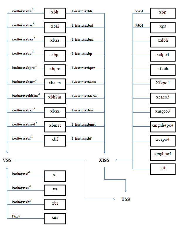
Figure 4‑8 - MANTIS2LIB - Calculation Procedure for Composite Variables VSS, TSS
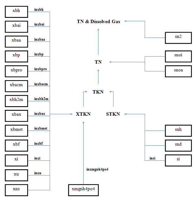
Figure 4‑9 - MANTIS2LIB - Calculation Procedure for Composite Variables STKN and TKN
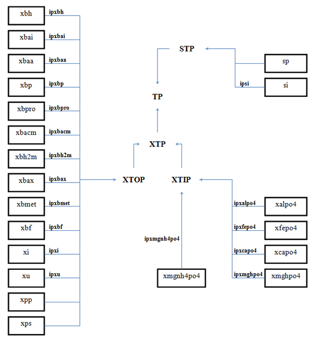
Figure 4‑10 - MANTIS2LIB - Calculation Procedure for Composite Variables STP, XTP, and TP
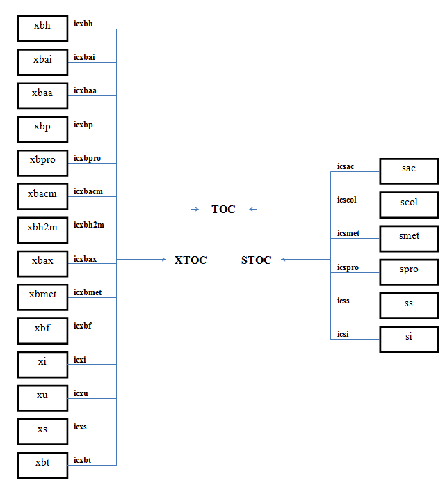
Figure 4‑11 - MANTIS2LIB - Calculation Procedure for Composite Variables STOC and TOC
All of the composite variables, including the most common ones such as X (total suspended solids), TKN (Total Kjeldahl Nitrogen), BOD, COD, etc., can be accessed by selecting the Output Variables > Concentrations menu. These variables (and those found by clicking on the More... button) can be tagged and placed on output graphs.
Whether stoichiometry has been set globally or locally within each object, the list of composite variables that are available to be displayed will depend on which library has been used for that particular GPS-X layout (CNLIB, CNPLIB, etc.).
It is possible to use a model in the layout that does not simulate the fate of all components of a given library (e.g. mantis in CNPLIB, which does not model phosphorus even though there are phosphorus state variables in CNPLIB). In these cases, these extra components will be modelled as if they were inert (i.e. no biological transformation applied, but mixing and settling are applied).
The composite variable list displayed in the Output Variables > Concentrations menu is the list associated with the library used to create the layout (e.g. CNPLIB). All composite variables are calculated for the given library, even if the component states are not modelled biologically in the reactor. For the example above (mantis model in CNPLIB), soluble phosphorus (sp) is not modelled biologically, and therefore behaves the same as si (soluble inerts); however, because CNPLIB contains the composite variable TP (total phosphorus), it will be calculated (from sp and other components) even though sp was modelled as an inert.
It is important to take this into consideration when selecting which model and library you will be using when creating your plant layout.
For every influent model that is used in a wastewater plant layout, it is important to properly specify the influent characteristics and the influent stoichiometry.
To help users better understand influent characterization, a special utility program, called Influent Advisor, was developed by Hydromantis. The tool helps users to visualize and debug influent characterization data. It is recommended that users make use of this utility tool so that influent characterization errors can be avoided.
The mathematical description of the influent wastewater that is fed to the plant model is the single most important aspect of a simulated system. Without significant consideration of the influent characterization, the plant model will be limited in its ability to predict the dynamic behavior of the plant.
To access the Influent Advisor tool, right-click on any wastewater influent object, and select the Composition > Influent Characterization menu item.
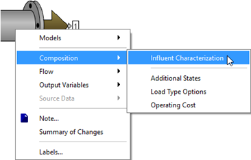
Figure 5‑1 - Opening the Influent Advisor Tool
The Influent Advisor screen shows three columns of data: User Inputs, State Variables, and Composite Variables, as shown in Figure 5‑2.

Figure 5‑2 - Influent Advisor Menu
The fields in the left-hand column show the inputs available to the user, such as influent concentrations and stoichiometric ratios. The centre and right hand columns show the state variable and composite variable concentrations calculated from the user inputs.
As the user changes values in the left-hand column, the variables in the centre and right-hand columns are automatically updated. This allows for easy debugging of confusing or conflicting influent characterization data.
Clicking on any variable in the centre and right-hand column illustrates how that value is calculated. The formula will be displayed in the formula box (located in the lower middle of the screen – you may need to scroll down to see it). The values used in the formula will be highlighted in the tables so that the applicable cells can be identified. If a negative value is calculated in either table, the cell will turn red. Correcting problematic data is only a matter of adjusting the input cells to achieve non-negative values.
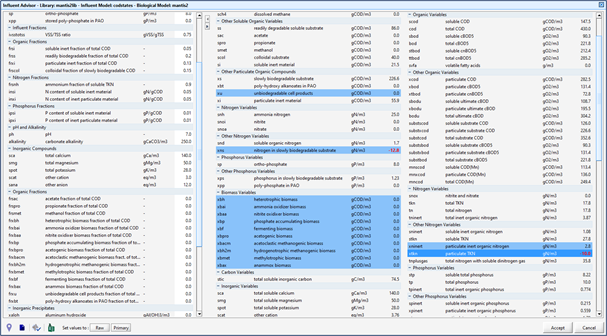
Figure 5‑3 -
Influent Advisor Screen Showing Highlighted Cells and Negative
Values
(Highlighted in Red)
The influent models used in GPS-X make certain assumptions about what data may or may not be available. For instance, no influent model uses both COD and BOD data, even though this data may be available and may provide important information about how that organic material is partitioned into the available state variables. Influent Advisor helps overcome this shortcoming.
Take an example in which BOD and COD data is available and the BODbased model is chosen for the influent object. The applicable data can be entered into Influent Advisor, including the available BOD data. The user can then scroll to the right table and check the COD value calculated based on the input data. If the COD data is in agreement with the measured COD data (assuming no negative values in any cells), then the user can be assured that the input data is consistent with the available data. If the COD data is different from the measured COD, then the unknown (or estimated) input data should be adjusted until acceptable agreement is achieved.
NOTE: Correctly setting up the influent is critically important to the simulation; therefore, a set of warning messages has been developed, and will appear in the Command window, when necessary. For instance, if the user inadvertently enters a value for xsto, but has chosen ASM1 as the local biological model, then a warning message (`time = <timestamp> xsto<streamlabel> is non-zero, xsto is not a state variable in ASM1') will appear in the Log window. This is a signal to go back to the influent data forms and correct a problem with the influent. It is recommended that Influent Advisor be used to debug your influent characterization. Hydromantis recommends that users make full use of the Influent Advisor as a tool to help identify problems, and understand the interconnectivity between state and composite variables.
During a simulation, error messages related to the influent may appear in the simulation Log window. These messages will most likely be the result of improper influent stoichiometry. If an error message does appear, then the influent stoichiometry should be examined for possible errors.
There are five (5) influent objects in GPS-X:
Table 5‑1 – Influent Objects
|
Name |
Object |
Use |
Models Available |
|
Wastewater Influent |
|
Continuous wastewater flows (steady or dynamic) |
bodbased codbased codstates sludge states tssfrac |
|
Batch Influent |
|
Batch deliveries of septage or other discontinuous wastewater flows |
bodbased codbased codstates sludge states tssfrac |
|
Water Influent |
|
Clean water input (steady or dynamic) |
water |
|
COD Chemical Dosage |
|
Dosage of COD into streams or objects |
codfeed |
|
Acid Dosage |
|
Dosage of acid for pH control |
acidfeed |
The influent objects contain models, options, and features that are relevant to the type of influent being used. For example, the continuous wastewater model has options for specifying a diurnal pattern for influent flow, a feature not found in the chemical dosage object.
The wastewater influent object (brown arrow) is used to characterize continuous streams of wastewater flow. The continuous influent flow rate is specified in the influent object’s Flow > Flow Data menu. (Figure 5‑4 and Figure 5‑5)
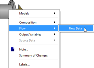
Figure 5‑4 - Selecting the Influent Flow Data Menu
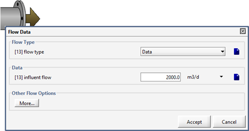
Figure 5‑5 - Influent Flow Data Menu, showing Flow Type Options
The flow is specified via one of the four methods:
1. Data – users set the flow rate directly, via menu entry or read from file.
2. Sinusoidal – GPS-X applies a sinusoidal curve to the influent flow set in the menu or read from file.
3. Diurnal Flow – a daily diurnal patter is set via flow rates at different times of the day.
4. Diurnal Flow Factor – a daily diurnal pattern is set via flow rates at different times of the day.
The influent models available in GPS-X depend on the model library and the local biological model used to relate the state variables to the composite variables. The manner in which the state variables are calculated sometimes differs from model to model and library to library. This chapter discusses the models available and the flow choices available with the batch influent object.
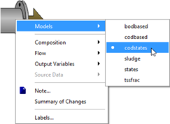
Figure 5‑6 -
The Influent Models
Each influent model calculates a complete set of library-dependent state variables that are passed to the rest of the plant layout. The influent models differ only in the type of information required as inputs to the model.
The descriptions of the influent models that follow are an overview of how they work; however, due to their complexity and their dependence on the local biological model, and the library currently in use, users are referred to the Influent Advisor to understand the calculations being made in each model.
The BODbased influent model is the choice when BOD data is available and COD data is not available; however, due to the approximations and the nature of the BOD measurement, special care must be taken to properly estimate influent particulate inerts. If this model is selected, the user inputs total carbonaceous BOD5, total TKN, total suspended solids, a few state variables. The state variables are normally zero, except for the soluble inert organics, soluble ortho-phosphate (CNPLIB) and alkalinity (Figure 5‑7 and Figure 5‑8 and several stoichiometric fractions).
These inputs are used to calculate the remaining influent state variables: readily biodegradable substrate (ss), slowly biodegradable substrate (xs), particulate inert organics (xi), free and ionized ammonia (snh), particulate biodegradable organic nitrogen (xnd), and soluble biodegradable organic nitrogen (snd).
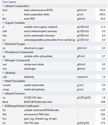
Figure 5‑7 – MANTIS2 Library BODbased Influent Model Inputs
The relationships between the calculated state variables and the composite and stoichiometric fractions are library-specific and the relationships are shown in the appendix to this chapter (Figure 5‑23 and Figure 5‑24). BODultimate is assumed to be equivalent to the biodegradable COD.
The stoichiometric fraction fss (soluble substrate:BODultimate), is used to determine what fraction of the total BODultimate is soluble substrate (sf for asm2d orss for all other biological models). In terms of sampling measurements, the fraction fss can be estimated from the ratio of filtered BOD20 :BOD20. The particulate substrate state variable (xs) is then calculated by difference (i.e. in cnlib, xs = BODultimate * (1-fss) -xba-xbh-xsto)). The particulate inert organics (xi) state variable is calculated by subtracting all the other particulate carbonaceous organic states (xsto, xbh, xba, xu (all input by user) and xs (calculated above)) from the particulate COD (XCOD).
Calculation of the three unknown nitrogen state variables depends on the calculation of TKN which is biological model-dependent. For instance, with the asm1 or mantis models the amount of free and ionized ammonia (snh) is the fraction of ammonia (fnh)multiplied by the TKN. The remainder is the biodegradable organic nitrogen, which is partitioned into three areas including nitrogen associated with particulate state variables (i.e. xbh, xba, xi and xu), and soluble and particulate organic nitrogen (snd and xnd) using the fxn fraction and the nitrogen fractions of the particulate state variables (Figure 5‑8).
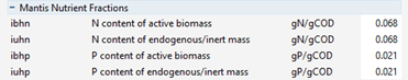
Figure 5‑8 – MANTIS2 Library Nutrient Fractions for the BODbased Influent Model
This differs from the calculations made when asm3 has been chosen as the local biological model because snd and xnd are not state variables in asm3. In this case, soluble TKN is calculated as the difference between the total TKN and the particulate TKN. The nitrogen associated with the soluble state variables (ss and si) is subtracted from the soluble TKN and the remaining TKN is equated to ammonia (snh). Hence, in the asm3 BOD based influent model, fnh and fxn are not used. Influent Advisor will help users determine what parameters are necessary for each mode.
This model requires an input of total COD, total TKN, total phosphorus (in CNPlib), state variables (the state variables are normally zero except for ammonia, soluble ortho‑phosphate and alkalinity) and several stoichiometric fractions. From these inputs, the complete set of state variables, composite variables and nutrient fractions are calculated (Figure 5‑18 and Figure 5‑19).
The calculation of the nitrogen and phosphorus (CNPlib) state variables and fractions is complicated in the codfractions influent models. This is because some of the nitrogen and phosphorus in the influent is associated with the organic state variables.(i.e. N content of active biomass). Therefore, the model must adjust itself depending on the applicable composite variable model and the current organic states. As with the other influent models, these nutrient fractions are specified in this model. However, in the event that a mass balance is not achievable with the user input data, the codfractions model will recalculate these nutrient fractions to force the mass balance. It is recommended that Influent Advisor be used to set-up and understand these calculations.
This model has the advantage that each of the calculations is based on the total COD, total TKN, total phosphorus (CNPlib), soluble ortho-phosphate (CNPlib) and ammonia inputs. Therefore, (as often is available in practice) a series of these data over a period of time can be read in from a data file and the influent state variables will vary with the load. This is in contrast to other influent models in which some state variables are input directly and will not automatically vary with a load change.
This model works similarly to the codfractions influent model, however all COD input fractions are set as a fraction of total COD. This allows users to specify total COD, TKN and ammonia as their main characterization inputs. Soluble inert COD (si), readily biodegradable substrate (ss, sf or slf), particulate inert material (xi), unbiodegradable cell products (xu) and biomass concentrations (xbh, xba and xbp) are specified via fractions of total COD, as shown in Figure 5‑9.
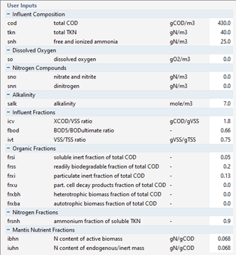
Figure 5‑9 - CODstates Influent Model Inputs
This model has been designed to mimic the input of a sludge stream. The user inputs the total suspended solids, a few state variables, and a couple of stoichiometric fractions. From these inputs, the organic solids are partitioned into heterotrophic biomass (i.e. degradable particulate material), polyphosphate accumulating biomass (CNPLIB only) and un-biodegradable particulate material. The remaining particulate organic state variables are set to zero. All the soluble state variables are defaulted to zero in this model, except for dissolved oxygen and alkalinity.
This model is appropriate if a full influent characterization has been performed and the influent state variables have been calculated manually. If the user selects the states model, input values for the state variables, and a few stoichiometric fractions used for calculating the composite variables are required. The CNlib states data entry form (Composition > Influent Composition) is shown in Figure 5‑9, and the stoichiometry entry form (Composition > Influent Stoichiometry) is shown in Figure 5‑10.
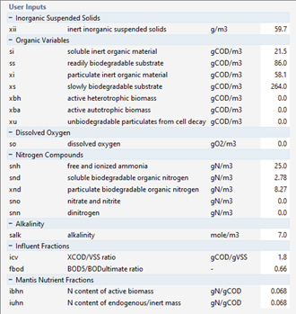
Figure 5‑10 - CN Library States Influent Model Influent Stoichiometry Inputs
The tsscod influent model can be used successfully if the influent was characterized using COD and suspended solids as the main components. The tsscod influent model was developed based on the Activated Sludge Model No. 2 report (Henze et al., 1995).
If this model is selected, the user inputs total COD, total TKN, total suspended solids, a few state variables (the state variables are normally zero except for the soluble inert organics, soluble ortho-phosphate (CNPLIB) and alkalinity and several stoichiometric fractions. These inputs are then used to calculate the remaining state variables (Figure 5‑7 and Figure 5‑8).
Particulate COD (XCOD) is calculated from the TSS using two stoichiometric fractions. This is then divided into its component parts via stoichiometric fractions or explicitly as read from the data input forms leaving the particulate inert organics component (xi) to be calculated by subtraction. Figure 5‑12 shows how the soluble COD (SCOD) components are calculated from the COD, XCOD and the stoichiometric parameter, frsi. See the bodbased model for the calculation of the nitrogen and phosphorus (CNPLIB) state variables. It is recommended that Influent Advisor be used to understand these calculations.
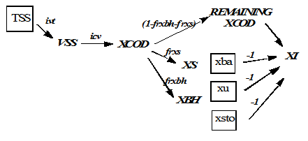
Figure 5‑11 - CN Library tsscod Model Particulate Inert Calculation
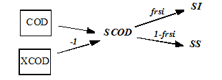
Figure 5‑12 - CN Library tsscod Influent Soluble Components Calculation
The runoff flow model uses a parallel linear reservoir model to simulate wet weather flow in sanitary and combined sewer systems. This model is not a mechanistic hydrological model, but a simple mathematical transformation.
The equations are:
Equation 5.1
![]()
and
Equation 5.2
![]()
where:
Pd = rainfall that enters the sewer system directly
Pi = rainfall that enters the sewer system indirectly
Ptotal = total rainfall over the catchment area
Cd = fraction of total rainfall that enters the sewer system directly
Ci = fraction of total rainfall that enters the sewer system indirectly
Total runoff (Qtotal) is calculated with the following equation:
Equation 5.3
![]()
which is based in the following equations:
Equation 5.4
![]()
Equation 5.5
![]()
Equation 5.6
Equation 5.7
![]()
where:
Kd = decay rate of linear reservoir representing direct runoff
Ki = decay rate of linear reservoir representing indirect runoff
A = total catchment area
The chemical dosage influent object (blue arrow) is used to characterize streams which are not typical wastewater inputs, but rather chemical or water inputs to a wastewater treatment process. The models found in the chemical dosage influent have been developed specifically for this purpose, and are set up for easy conversion of typical chemical components into the state variables used in the biological models. The flow is specified only through the Data option as described in Figure 5‑5.
The acetate influent model can be used to simulation the addition of acetate to the treatment process. The acetate dose (as acetic acid) can be entered as a percentage of purity, or in a variety of units (mol acetate/L, g (acetate*COD)/m3, g(acetate)/L, etc.), by selecting from the drop-down units menu (Figure 5‑13). The COD equivalent of the acetate dose is automatically converted to slf if asm2d or newgeneral have been chosen for the local biological model or ss (readily biodegradable substrate) for all other local biological models.
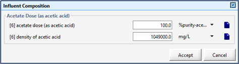
Figure 5‑13 - CN Library Acetate Influent Model - Acetate Dose Form
The methanol influent model can be used to simulate the addition of methanol to the treatment process. The methanol dose can be entered as a percentage of purity, or in a variety of other units (mol methanol/L, g(methanol*COD)/m3, g(methanol)/L, etc.), by selecting from the units drop-down menu (Figure 5‑14). The COD equivalent of the methanol dose is automatically converted to sf if asm2d has been chosen for the local biological model or ss (readily biodegradable substrate) for all other local biological models.
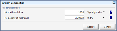
Figure 5‑14 - CN Library Methanol Influent Model Inputs
This influent model was developed to simulate a rain event or alkalinity addition whereby the influent hydraulic load could be increased without increasing the organic or nitrogen load to the plant. In the water influent, the only variable to be provided in the composition menu is the alkalinity. All other state variables are set to zero.
The difference between the batch influent (truck) object and the continuous influent objects (arrows) concerns the flow and load types. The available flow and load types for the batch influent object are averageand individual.
In the batch influent, if the average flow and load types are selected, the model will behave exactly like the continuous influent.
If the individual flow type is selected, there will be an intermittent (or batch) influent. Under the Flow sub-menu item individual, the user can specify the starting and ending time of the batch influent, and the volume of each truck (1 truck per day by default - the number of trucks per day is specified in the Influent Composition sub-menu). The total volume specified will be fed at an average rate over the total dumping time specified, that is there will be one influent flow spike.
If the individual load type is selected, the loading is determined by the amount specified in the Individual Loadssub-menu. The stoichiometry is specified in the Influent Characterizationmenu and the number of trucks per day is specified in the Compositionsub-menu (see Figure 5‑15).
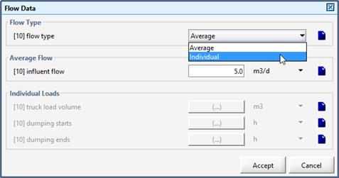
Figure 5‑15 - Batch Input Menu - Flow Data Model Inputs
When setting up your influent model, it is important that you realize what state variables are used in each biological model. The following sections outline the state variables used in the models in the different libraries.
Of similar importance is an understanding of how the composite variables are calculated from the state variables. This is important because many of the influent models go backwards (i.e. from the composite variables to the state variables); hence, an understanding of these relationships will help if debugging is necessary. Influent Advisor has been developed specifically to help navigate the more complicated influent models. The following figures were developed to help with this understanding.
The composite variable figures are copies of the figures presented in the composite variables chapter of this Reference; however, they are repeated here because of their importance to the influent model calculations.
This section contains one table and two figures which are to help the user understand how GPS-X has calculated the CNLIB state variables, and what state variables should be calculated depending on which biological model you are using.
Table 5‑2 - State Variables Used in Each Biological Model Included in CNLIB and CNIPLIB
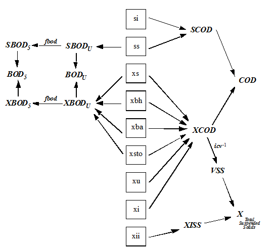
Figure 5‑16 – CN Library Organic State and Composite Variables
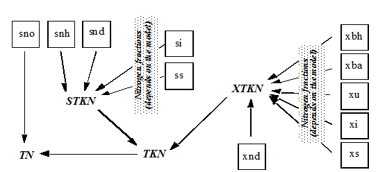
Figure 5‑17 - CN Library Nitrogen State and Composite Variables
This section contains one table and three figures which are to help the user understand how GPS-X has calculated the CNPLIB state variables, and what state variables should be calculated depending on which biological model you are using.
Table 5‑3 – State Variables Used in Each Biological Model included in CNPLIB and CNPIPLIB
|
State Variable |
Mantis |
ASM1 |
ASM2d |
ASM3 |
NewGeneral |
|
si |
|||||
|
ss |
|||||
|
sf |
|||||
|
slf |
|||||
|
xi |
|||||
|
xs |
|||||
|
xu |
|||||
|
xbh |
|||||
|
xba |
|||||
|
xbp |
|||||
|
xbt |
|||||
|
xsto |
|||||
|
so |
|||||
|
sp |
|||||
|
xpp |
|||||
|
xppr |
|||||
|
snh |
|||||
|
snd |
✓ |
||||
|
xnd |
✓ |
||||
|
sno |
✓ |
||||
|
snn |
✓ |
|
|||
|
salk |
✓ |
✓ |
✓ |
||
|
xmeoh |
|
|
|
|
|
|
xmep |
|
|
|||
|
xii |
✓ |
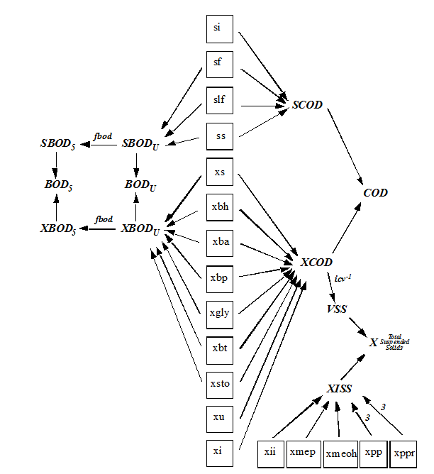
Figure 5‑18 - CNP Library Organic State and Composite Variables
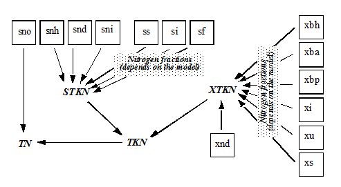
Figure 5‑19 - CNP Library Nitrogen State and Composite Variables
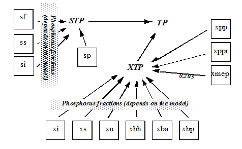
Figure 5‑20 - CNP Library Phosphorus State and Composite Variables
There are seven influent objects in MANTIS2LIB of GPS-X:
Table 5‑4 - Influent Objects in MANTIS2LIB
|
Name |
Object |
Use |
Models Available |
|
Wastewater Influent |
|
Continuous wastewater flows (steady or dynamic) |
bodbased
states |
|
Batch Influent |
|
Batch deliveries of septage or other discontinuous wastewater flows |
bodbased codbased codstates sludge states tssfrac |
|
Water Influent |
|
Clean water input (steady or dynamic) |
water |
|
Stormwater Runoff |
|
Clean water input from storm events |
runoff |
|
COD Chemical Dosage |
|
Dosage of COD into streams or objects |
codfeed |
|
Acid Dosage |
|
Acid addition for pH control |
acidfeed |
|
Alkali Dosage |
|
Alkali addition for pH control |
alkalifeed |
|
Nutrient Dosage |
|
Nutrient addition |
nutrifeed |
The eight influent objects contain models, options and features that are relevant to the type of influent being used. For example the continuous wastewater model has options for specifying a diurnal pattern for influent flow, a feature not found in the other influent objects. The influent models in MANTIS2LIB are similar to influent models in other libraries with a few differences.
The flow rate setup
in wastewater influent object is similar to the flow rate setup in
other libraries. The built-in influent advisor also works in a
similar way as for the other libraries. However, a few key
differences are with respect to how the stoichiometric parameters
for composite variable calculations are organized and calculated in
this library. In MANTIS2LIB, the stoichiometric parameters are
accessed through the
System > Input Parameters > Biochemical Model
Settings menu (Figure 5‑21). The
stoichiometric parameters available in the COD to VSS ratio
and Fractions Used in Composite Variable Calculations are
shown in Figure 5‑22 and Figure 5‑23.
The stoichiometric parameters available in the COD to VSS
ratio group are the parameters which are influent specific and
representative of a composite component of unknown composition. On
the other hand, the stoichiometry parameters available in the
Fractions Used in Composite Variable Calculations are
parameters which can be calculated based on the chemical
composition (acetic acid, methanol etc.) of the component or some
underlying fundamental estimation procedure. The default values of
inorganic fractions (N, P, etc.) in different type of biomass may
be accessed by pressing the More… button on the Fractions
Used in Composite Variable Calculations group (Figure
5‑24).
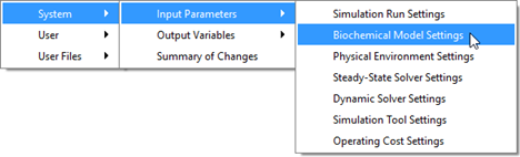
Figure 5‑21 - Accessing the Stoichiometry Parameters in MANTIS2LIB
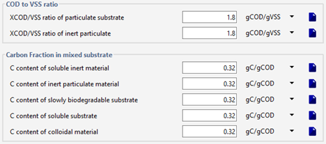
Figure 5‑22 - Influent Specific Stoichiometric Parameters
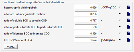
Figure 5‑23 - Fixed Stoichiometric Parameters in MANTIS2LIB
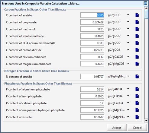
Figure 5‑24 - More... Fixed Stoichiometric Parameters in MANTIS2LIB
The batch influent object in MANTIS2LIB is similar to the batch influent object in other libraries.
The water influent object is similar to the batch influent object in other libraries.
The COD chemical dosage object uses the codfeed model (Figure 5‑25). The COD chemical dosage object allows user to select the type of COD used in the feed. Six COD sources acetic acid, propionic acid, methanol, molasses, glycerol and generic mixed substrate are available for selection from the Composition > Feed Chemical Details menu (Figure 5-26). The Feed Chemical Details menu is as shown in Figure 5‑27.
For pure organic chemical acetic acid, propionic acid, methanol and glycerol, two input parameters of % purity and density of chemical solution at the selected %-purity are required as input. Depending on the chemical selection, the concentration of the corresponding state variable is set. For example, if acetic acid is selected, the concentration of acetate (sac) is set to the value determined by the set % purity and density of the chemical solution. For molasses and mixed substrate, in addition to the density and % purity of the compound, N/COD and P/COD ratios in the substrate may be specified by the user. The nitrogen compound in the substrate is assigned to the soluble organic nitrogen state variable (snd) while the phosphorus in chemical is assigned to the soluble ortho-P state variable (sp).
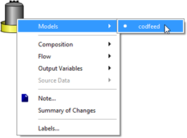
Figure 5‑25 - Models in COD Chemical Dosage Influent Object
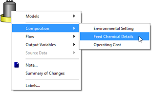
Figure 5‑26 - Accessing Feed Chemical Details Menu
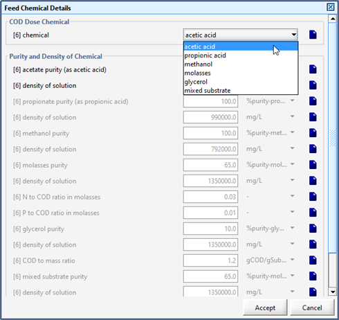
Figure 5‑27 - Selection of Feed Chemical and Set-up of Chemical Properties
The COD chemical dosage object has a built-in flow rate controller. The controller is useful for controlling the feed rate of COD based on a user defined controlled variable.
The acid dosage object is only available in the MANTIS2LIB. The acid dosage object uses the acidfeed model (Figure 5‑28). The acid dosage object allows user to select the type of acid used in the feed. Three acids HCl, H2SO4 and HNO3 are available for selection from the Composition > Feed Chemical Details menu (Figure 5‑29). The Feed Chemical Details menu is as shown in Figure 5‑30. For the selected chemical, two input parameters of % purity and density of chemical solution at the selected %-purity are required. If HCl or H2SO4 is selected, the state variable of other anion (sana) is set to the equivalent dosed amount. If HNO3 is the selected acid then, the state variable of Nitrate-N (snoa) is set to an equivalent concentration.

Figure 5‑28 - Models in Acid Dosage Influent Object
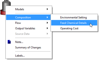
Figure 5‑29 - Accessing Feed Chemical Details Menu
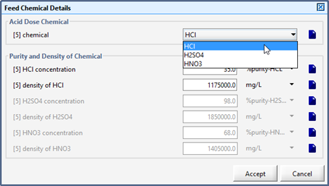
Figure 5‑30 - Selection of Feed Chemical Set-up of Chemical Properties
The acid dosage object has a built-in flow rate controller. The controller is useful for controlling the feed rate of acid based on a control variable (i.e. pH) in a reactor of interest.
The alkali dosage object is only available in the MANTIS2LIB. The alkali dosage object uses the alkalifeed model (Figure 5‑31). The alkali dosage object allows user to select the type of alkali (base) used in the feed. Six alkalis NaOH, Ca(OH)2, Mg(OH)2, NaHCO3, CaCO3 and Na2CO3 are available for selection from the Composition > Feed Chemical Details menu (Figure 5‑32). The Feed Chemical Details menu is as shown in Figure 5‑33. For the selected chemical, two input parameters of % purity and density of chemical solution at the selected %-purity are required. The chemical and corresponding state variables which are set in the feed are shown in Table 5‑5.
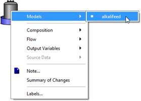
Figure 5‑31 - Models in Alkali Dosage Influent Object
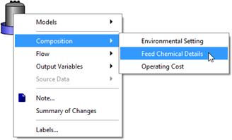
Figure 5‑32 - Accessing Feed Chemical Details Menu
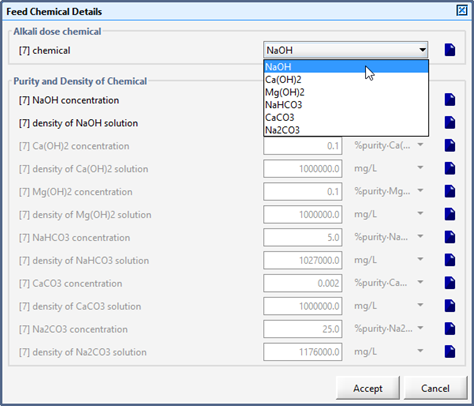
Figure 5‑33 - Selection of Feed Chemical and Setup of Chemical Properties
Table 5‑5 - Alkali Chemicals and Affected States in the Feed
|
Chemical |
Affected States in Feed |
|
NaOH, |
sana |
|
Ca(OH)2, |
sca |
|
Mg(OH)2, |
smg |
|
NaHCO3 |
sana, stic |
|
CaCO3 |
sca, stic |
|
Na2CO3 |
sana, stic |
The alkali dosage object has a built-in flow rate controller. The controller is useful for controlling the feed rate of alkali based on a control variable (e.g. pH) in a reactor of interest.
The nutrient dosage object is only available in the MANTIS2LIB. The nutrient dosage object uses the nutrifeed model (Figure 5‑34). The nutrient dosage object allows user to select the type of nutrient used in the feed. Four nutrients NH4Cl, Urea, (NH4)3PO4 and H3PO4 are available for selection from the Composition > Feed Chemical Details menu (Figure 5‑35). The Feed Chemical Details menu is as shown in Figure 5‑36. For the selected chemical, two input parameters of % purity and density of chemical solution at the selected %-purity are required. The chemical and corresponding state variables which are set in the feed are shown in
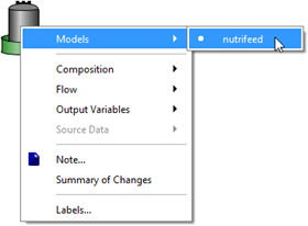
Figure 5‑34 - Models in Nutrient Dosage Influent Object

Figure 5‑35 - Accessing Feed Chemical Details Menu

Figure 5‑36 - Selection of Feed Chemical and Setup of Chemical Properties
Table 5‑6 - Nutrient Chemicals and Affected States in the Feed
|
Chemical |
Affected States in Feed |
|
NH4Cl |
snh, sana |
|
Urea |
snd |
|
(NH4)3PO4 |
snh, sp |
|
H3PO4 |
sp |
|
MgCl2 |
smg, sana |
The nutrient dosage object has a built in flow rate controller. The controller is useful for controlling the feed rate of nutrient for a user-defined control variable.
This chapter examines the suspended-growth models that are available in the different GPS-X libraries. Each of the biological models available in GPS-X is implemented in both the completely mixed and plug-flow formats in many different unit process objects. The biological model is the same, however, regardless of the hydraulic implementation.
Before discussing specific models, some common features are presented:
The oxygen transfer model is based on theory presented in the USEPA Design Manual for Fine Pore Aeration Systems (USEPA, 1989) and Mueller et al. (2002). The GPS-X aeration model is suitable for accurate design of diffused and surface mechanical aeration systems.
In GPS-X, oxygen transfer to the bulk liquid phase of a biological reactor is modelled using a dynamic mass balance written for dissolved oxygen gas. For example, a dissolved oxygen mass balance around a completely stirred tank reactor (CSTR) is shown below in Equation 6.1.
Equation 6.1
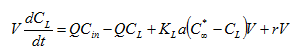
where:
V = reactor volume (m3)
CL = concentration of dissolved oxygen (DO) in the reactor (mg/L)
Q = influent flow rate (m3/d)
Cin = concentration of DO entering reactor (mg/L)
KLa = oxygen mass transfer coefficient at field conditions (1/day)
C*∞ = DO saturation concentration at field conditions (mg/L)
r = rate of use of DO by biomass (g/day), the respiration rate
The volume flows, and reaction rates are known from specifications or other modelling equations leaving two terms that must be calculated in order to solve the dissolved oxygen mass balance over time for the DO concentration in the reactor, CL:
1. DO saturation concentration at field conditions, C*∞, and,
2. Oxygen mass transfer coefficient at field conditions, KLa
The DO saturation concentration at field conditions is calculated as follows:
Equation 6.2
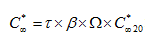
where:
τ = temperature correction factor (unitless)
β = correction factor for salts, particulates, and surface-active substances (unitless)
Ω = pressure correction factor (unitless)
C*∞20 = DO saturation concentration at 20°C and 1 atm (mg/L)
The correction factors are used to adjust the DO saturation concentration to account for the temperature of the liquid, the pressure at the submergence level of the diffusers, and the salts, precipitates, and surface-active substances found in the wastewater.
The temperature correction factor is calculated as follows:
Equation 6.3

where:
C*st = surface DO saturation concentration at temperature of t and 1 atm (mg/L)
C*s20 = surface DO saturation concentration at 20°C and 1 atm (mg/L)
The surface DO saturation concentration at liquid temperature t and a pressure of 1 atm is obtained using a lookup table in GPS-X that is based on temperature. The lookup table data were taken from Appendix C of the USEPA Design Manual – Fine Pore Aeration Systems (USEPA, 1989). When the temperature falls between two data points in the table, GPS-X uses linear interpolation to determine the C*st value. The value of C*s20 is 9.09 mg/L.
The correction factor for salts, particulates, and surface-active substances β, is a parameter that must be measured or estimated for the wastewater of interest. In GPS-X, a default value of 0.95 is used.
The pressure correction factor is calculated as shown below:
Equation 6.4
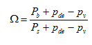
where:
Pb = barometric pressure at elevation and air temperature (kPa)
Ps = standard barometric pressure (101.325 kPa)
pv = vapour pressure of water at liquid temperature (kPa)
pde = effective pressure at depth of diffuser submergence
The barometric pressure at elevation and air temperature is calculated using the following formula taken from Appendix B-2 of Metcalf and Eddy (2003):
Equation 6.5
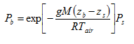
where:
g = acceleration due to gravity (9.81 m/s2)
M = molecular weight of air (28.964 kg/kg-mole)
R = universal gas constant (8314 m/kg-mole K)
Tair = air temperature (K)
zi = elevation at position i (m)
The vapour pressure of water at the liquid temperature is determined using the Antoine equation (Felder & Rosseau, 1986):
Equation 6.6
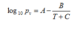
where:
A, B, C, = Antoine
coefficients
(found in System > Input Parameters >Physical
form in GPS-X under Physical Constants)
T = wastewater temperature (°C)
The effective pressure at the depth of the diffuser submergence is calculated using the following formula:
Equation 6.7
![]()
where δ is the depth correction factor for oxygen saturation and is given by:
Fine Pore and Jets
Equation 6.8
![]()
Coarse Bubble
Equation 6.9
![]()
The parameter d is the depth of submergence of the diffusers.
The DO saturation concentration at 20°C and 1 atm is calculated as follows:
Equation 6.10
![]()
The value of the
oxygen mass transfer coefficient at field conditions,
KLa, specifies the amount of oxygen supplied to
the aeration tank given the driving force![]() ,
and the tank volume. GPS-X provides four ways for the user to
specify the KLa:
,
and the tank volume. GPS-X provides four ways for the user to
specify the KLa:
1. If known, the user can directly supply the KLa at 20°C (no alpha, fouling, or temperature correction) for both diffused and mechanical aeration. GPS-X converts the KLa to field conditions.
2. In the case of mechanical aerators, the user can supply an aeration power and mechanical aerator oxygen transfer rate from which GPS-X calculates the KLa.
3. In the case of diffused aeration, the user can supply an air flow rate (at either standard or field conditions) and a standard oxygen transfer efficiency (SOTE) from which GPS-X calculates the KLa at field conditions.
Alternatively, the user can configure a DO controller which will manipulate the field KLa directly to match the desired DO concentration. The availability of these options depends on the selected aeration method. For diffused aeration the user can enter airflow, enter KLa, or use a DO controller. For mechanical aeration the user can enter power, enter KLa, or use a DO controller. The four choices for specifying KLa are discussed in more detail in the following four sections.
Entering KLa Directly – Diffused Aeration
The KLa at field conditions is calculated using Equation 6.11:
Equation 6.11
![]()
where:
KLaT = mass transfer coefficient at temperature T in °C (1/day)
KLa20 = mass transfer coefficient at 20°C
θ = temperature correction factor (default value in GPS-X is 1.024)
α = wastewater correction factor for KLa20
F =diffuser fouling factor (default value in GPS-X is 1.0)
T = wastewater temperature (°C)
The αcorrection factor can be specified along the length of the aeration tank in the case of a plug flow unit process.
GPS-X calculates other useful process variables from the standard and field KLa as detailed below:
Oxygen Transfer Rate (OTR) at Field Conditions in g/d
Equation 6.12
![]()
Standard Oxygen Transfer Rate (SOTR) in g/d
Equation 6.13
![]()
Airflow at Standard Conditions in m3d
Equation 6.14
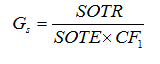
where:
SOTE = standard oxygen transfer efficiency (as a fraction)
CF1
= conversion factor to account for the density, molecular weight,
and O2 mole fraction of the standard air
(U.S. Standard = 277.6533841; European Standard = 300.495893)
In the case of user-defined standard air (see Entering Airflow section below), the airflow is calculated using Equation 6.15.
Equation 6.15
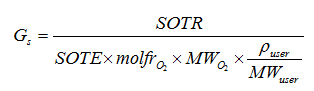
where:
molfrO2 = mole fraction of O2 in user-defined air (mole/mole)
MWO2 = molecular weight of O2 (32 g/mole)
Puser = density of user-defined air (g/m3)
MWuser = average molecular weight of user-defined air (g/mole)
The airflow at either U.S. or European standard conditions is converted to field conditions using the ideal gas law:
Equation 6.16
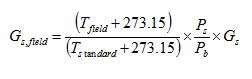
where:
Tstandard = air temperature at standard conditions (°C)
Tfield = air temperature at field conditions (°C)
Equation 6.16 assumes that the field air has the same humidity as the standard air. If the humidity of the field air is different than for the standard air, the user can multiply the GPS-X calculated field air by the ratio of the mole fraction of oxygen in the field air by the mole fraction of air in the standard air.
No conversion to field conditions is undertaken for user-defined standard air.
Mechanical surface aeration is calculated similarly to diffused; however, the fouling and depth correction factors are not required and oxygen transfer is related to the mechanical power input.
For mechanical surface aeration, the formula for the DO saturation concentration at field conditions is modified as follows:
Equation 6.17
![]()
as δ = 1 in this case, the pressure correction factor is re-defined as:
Equation 6.18
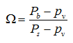
The KLa at field conditions is calculated using Equation 6.19.
Equation 6.19
![]()
The OTR is calculated using Equation 6.20 as shown below:
Equation 6.20
![]()
The SOTR is calculated as follows:
Equation 6.21
![]()
The mechanical power is calculated using the SOTR:
Equation 6.22
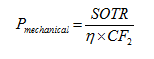
where:
Pmechanical = mechanical power (kW)
η = mechanical aerator oxygen transfer rate (1.75 kg O2/kW h)
CF2 = conversion factor (24,000)
The default α value for mechanical aeration in GPS-X is 0.9.
The airflow can be entered at either standard or field conditions. At standard conditions, the user has three options:
1. U.S. Standard Conditions:
a. Temperature = 20°C
b. Pressure = 1 atm
c. Relative humidity = 36%
2. European Standard Conditions:
a. Temperature = 0°C
b. Pressure = 1 atm
c. Relative humidity = 0%
3. User-Defined Standard Conditions:
The user must specify the properties (mole fraction of O2 in air, density, molecular weight, and exponent in blower power equation). When using the user-defined standard conditions option, GPS-X uses a Henry’s law correction to adjust the value of C*st.
Equation 6.23
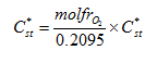
GPS-X converts the airflow to U.S. standard conditions and then calculates the SOTR using Equation 6.13. The OTR is calculated using Equation 6.24.
Equation 6.24
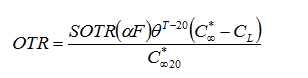
The oxygen mass transfer coefficient at field conditions is calculated using Equation 6.11. If the airflow is entered at U.S. or European standard conditions, the airflow at field conditions is calculated using Equation 6.16.
If mechanical power is entered, the SOTR in g/d is calculated using Equation 6.21. The KLa at field conditions is then calculated using Equation 6.19 and the OTR is calculated using Equation 6.20.
The user has the option of controlling the aeration supply to the reactor to maintain a specific dissolved oxygen setpoint. In this case the model will calculate the necessary oxygen mass transfer coefficient at field conditions to maintain the DO at the setpoint.
For diffused aeration with DO control, GPS-X uses Equation 6.12, Equation 6.13, and Equation 6.14 to calculate the SOTR, OTR, and airflow. For mechanical aeration with DO control, GPS-X uses Equation 6.20, Equation 6.21, and Equation 6.22 to calculate the OTR, SOTR, and mechanical power
The user has the option of using a constant SOTE or using a correlation in GPS-X to calculate the SOTE. When using the constant SOTE option, the default value (0.3) represents a typical estimate of the efficiency for fine bubble diffusers submerged at 4.3 m (14 ft.).
Alternatively, GPS-X has SOTE correlations for fine bubble, coarse bubble, and jet diffusers. For fine bubble aeration, the SOTE correlations are based on a regression equation developed by Hur (1994) which is shown below:
Equation 6.25
![]()
where:
AF = air flow per diffuser (scfm per diffuser)
d = diffuser submergence (ft.)
DD = diffuser density (diffusers/100ft2)
A1, A2, A3, A4, and A5 = regression parameters
As shown, this equation depends on the depth of submergence of the diffusers, the diffuser density, and the airflow per diffuser. Using this equation and the data found in Hur (1994), Hydromantis re-estimated the regression parameters to improve the fit of the regression. Separate regressions were performed for ceramic disc, ceramic dome, membrane disc, and membrane tube diffusers. The values of the regression coefficients can be found in the System > Input Parameters > Physical > More form.
There is also an option to use a user-defined SOTE correlation. The correlation has the same form as Equation 6.25. The adjustable regression coefficients are found in the System > Input Parameters > Operational > More form of most biological objects.
A separate correlation for coarse bubble and jet diffusers has been developed by Hydromantis based on data found in Mueller et al (2002) as shown in Equation 6.26.
Coarse Bubble and Jet SOTE
Equation 6.26
![]()
The SOTE for coarse bubble and jet diffusers is dependent upon the airflow per diffuser and the diffuser submergence.
In all the SOTE correlations, the airflow per diffuser has been limited to be within the ranges used for calibration. The correlations are empirical and should not be extrapolated outside of the calibration range. The ranges are used as follows:
Fine Bubble
Ceramic Disc: 0.5 ≤ AF ≤ 5m3/h/diffuser
Ceramic Dome: 0.5 ≤ AF ≤ 4.4 m3/h/diffuser
Membrane Disc: 0.8 ≤ AF ≤ 5 m3/h/diffuser
Membrane Tube: 0.8 ≤ AF ≤ 15 m3/h/diffuser
Coarse Bubble
14 ≤ AF ≤ 58 m3/h/diffuser
Jet
8 ≤ AF ≤ 140 m3/h/diffuser
GPS-X applies a warning message to the log window if the airflow per diffuser is outside the ranges given above.
The fine bubble SOTE correlation is modified for tanks deeper than 8 m. Work by Pöpel and Wagner (1994) has shown that the SOTE does not continue to increase linearly with the depth of submergence beyond depths of approximately 8 m (see Figure 8 in Pöpel and Wagner (1994)). At depths greater than 8 m the SOTE starts to level off so that the SOTE can never be greater than 100 %.
An extra quadratic term in diffuser submergence is added to Equation 6.25 when the diffuser submergence is greater than 8 m, as shown in Equation 6.27.
Equation 6.27
![]()
The regression
parameter A6 can be accessed in GPS-X in the
Input Parameters > Operational > More
form. The parameter A6 was estimated by
Hydromantis uses linear regression to fit Equation
6.26 to the solid curve in Figure 8 of Pöpel and Wagner
(1994). In order to perform the regression it was
necessary to first adjust the airflow per diffuser and the diffuser
density to match the SOTE of 20 % at depth of 5 m shown in Figure 8
of Pöpel and Wagner (1994).
The deep tank SOTE correlation is only applied for fine bubble diffusers. It can be turned off by setting the parameter A6 to zero in GPS-X.
The wire power in kW consumed by the blowers in order to deliver the required air is calculated in GPS-X as follows:
Equation 6.28

where:
DP = delivered power of blowers (kW)
e = overall efficiency of mechanical equipment (i.e. blowers, motors, coupling, and gearbox)
The overall efficiency of the mechanical equipment is entered into GPS-X in the Input Parameters > Operating Cost form of most biological objects. The delivered power of the blowers is calculated using the adiabatic compression equation (Mueller et al., (2002)):
Equation 6.29
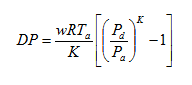
where:
w = mass flow rate of air
R = universal gas constant
Ta = blower inlet air temperature (degrees K)
K =
R/Cp where Cp is the heat
capacity of air at constant pressure
(K = 0.283 for U.S Standard Air and K = 0.2857 for
European Standard Air)
Pd = absolute pressure downstream of blower (discharge pressure in kPa)
Pa = absolute pressure upstream of blower (inlet pressure in kPa)
The discharge pressure of the blower is calculated as follows:
Equation 6.30
![]()
where:
Ps = barometric pressure (default is 101.325 kPa)
g = acceleration due to gravity (9.81 m/s2)
Δpd = pressure drop in piping and diffuser downstream of blower (found in Input Parameters > Operating Cost form of most biological objects)
The inlet pressure is calculated as shown in Equation 6.31
Equation 6.31
![]()
where:
Δpa = pressure drop in inlet filters and piping to blower (found in Input Parameters > Operating Cost form of most biological objects.)
This section discusses the aeration forms that are applicable to most biological objects. The forms from the Completely-Mixed Tank are used as an example.
The Aeration Setup form is accessed by right-clicking on most biological objects and selecting Input Parameters > Operational. Figure 6‑1 shows the GPS-X form. The parameters are discussed below:
Aeration method (Diffused Air/Mechanical (Surface Aeration)): Specifies whether the aeration system is diffused or mechanical (surface).
Specify oxygen transfer by… (1 Entering Airflow/2 Entering KLa/3 Entering Mechanical Power/4 Using a DO Controller): Specifies the method of oxygen transfer, entering airflow, KLa, mechanical power, or using a DO controller. Entries that do not apply are greyed out. For example, you cannot specify the oxygen transfer by entering mechanical power if the aeration method is diffused.
Oxygen mass transfer coefficient (clean water): Clean water KLa at 20°C with no alpha or fouling factor correction.
Air flow into aeration tank: Diffused air flow into the aeration tank. The airflow can be at standard conditions (U.S., European, or User-Defined) or at field conditions depending on user selections. The user can select standard or field conditions in the Input Parameters > Operational > More… form. The user can select which standard conditions are used in the Input Parameters > Physical >More… if local conditions for O2 solubility are used, or in the System >Input Parameters > Physical form if global conditions for O2 solubility are used.
Aeration power: The power of the mechanical aeration system.
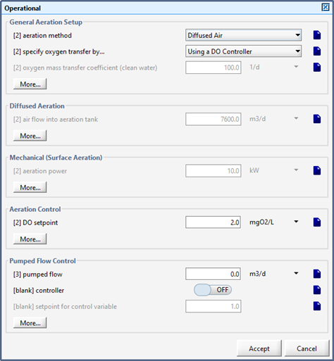
Figure 6‑1 - Aeration Setup Form in Operational Form
By clicking on the More… button, the form shown in Figure 6‑2 and Figure 6‑3can be accessed. The parameters found in this form are discussed in the subsequent sections.
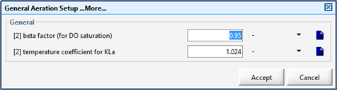
Figure 6‑2 - General Aeration Setup > More... Form
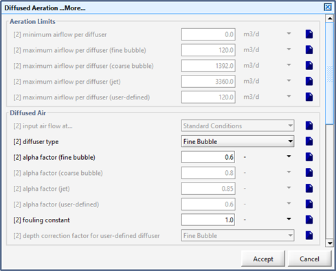
Figure 6‑3 - Diffused Aeration Setup > More... (Part 1)
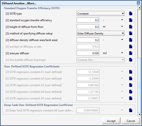
Figure 6‑4 - Diffused Aeration Setup > More... Form (Part 2)
Beta factor (for DO saturation): Specifies the DO saturation concentration correction factor for sales, particulates, and surface-active substances. The default value is 0.95.
Temperature coefficient for KLa: Specifies the temperature correction factor for KLa, θ (default value is 1.024).
Minimum oxygen mass transfer coefficient: Specifies the minimum value of the KLa at field conditions. GPS-X bounds the field KLa to be greater than or equal to this maximum in all cases.
Maximum oxygen mass transfer coefficient: Specifies the maximum value of the KLa at field conditions. GPS-X bounds the field KLa to be less than or equal to this maximum in all cases.
Mechanical aerator oxygen transfer rate: Specifies the mass of oxygen transferred to the liquid per unit of energy used by the mechanical aerator.
Alpha factor (mechanical aeration): Wastewater correction factor for mechanical KLa. The default value is 0.9.
Input air flow
at… (Field Conditions/Standard Conditions): Allows user
to specify whether the diffused air flow is entered at standard
conditions or field conditions. The user can select which
standard conditions are used in the
Input Parameters > Physical > More … if local
conditions for O2 solubility are used or in the
System > Input Parameters > Physical form if
global conditions for O2 solubility are used.
Diffuser type (Fine Bubble/Coarse Bubble/Jet/User-Defined): Specifies the type of diffuser to be used. This option is only active if diffused air has been selected. GPS-X uses this selection to select the appropriate alpha value and to select the appropriate SOTE correlation (if applicable).
Alpha factor (fine bubble): Specifies the value of the wastewater correction factor for the fine bubble KLa. The default value is 0.6.
Alpha factor (coarse bubble): Specifies the value of the wastewater correction factor for the coarse bubble KLa. The default value is 0.8.
Alpha factor (jet): Specifies the value of the wastewater correction factor for the jet KLa. The default value is 0.85.
Alpha factor (user-defined): Specifies the value of the wastewater correction factor for the user-defined KLa. The default value is 0.6
Fouling constant: Diffuser fouling factor. Default value is 1 (i.e. no fouling)
Depth correction factor for user-defined (Fine Bubble/Coarse Bubble): When the user-defined diffuser type is being used, this parameter selects whether Equation 6.8 or Equation 6.9 is used to calculate the depth correction factor for the DO saturation concentration.
SOTE type (Constant/Correlation): Specifies whether the SOTE is set by the user or calculated by a correlation. The correlation used depends on the diffuser type selected.
Standard oxygen transfer efficiency: When the SOTE type is set to constant, this value is used for the SOTE.
Diffuser submergence: Specifies the depth of submergence of the diffusers.
Method of specifying diffuser setup (Enter Number of Diffusers/Enter Diffuser Density): Allows the user to either specify the number of diffusers or the diffuser density (diffuser area/tank area). It is important to enter the diffuser density or the number of diffusers if an SOTE correlation is being used or the user requires GPS-X to display accurate values of the airflow per diffuser and the number of diffusers per unit area.
Diffuser density (diffuser area/tank area): When the method of specifying the diffuser setup has been selected as diffuser density, this parameter allows the user to enter the diffuser density as a fraction or a percentage. Diffuser densities between 5 % and 25 % are typical.
Number of diffusers or jets: When the method of specifying the diffuser setup has been selected as enter number of diffusers, this parameter allows the user to enter the number of diffusers.
Tank floor area: The area of the tank floor. It is important to enter the tank foor area if an SOTE correlation is being used or the user requires GPS-X to display an accurate value of the number of diffusers per unit area.
Area per diffuser: The floor area taken up by a diffuser. It is important to enter the area per diffuser if an SOTE correlation is being used and the user is entering the diffuser density. The default value is 0.038 m2 which is typical for a 9″ diameter ceramic diffuser.
Fine bubble diffuser head type (Ceramic Disc/Ceramic Dome/Membrane Disc/ Membrane Tube): Used to specify the fine bubble diffuser head type when fine bubble diffused aeration has been specified and an SOTE correlation is being used.
SOTE regression constant A1 (user-defined): Regression parameter A1 in user-defined SOTE correlation.
SOTE regression constant A2 (user-defined): Regression parameter A2 in user-defined SOTE correlation.
SOTE regression constant A3 (user-defined): Regression parameter A3 in user-defined SOTE correlation.
SOTE regression constant A4 (user-defined): Regression parameter A4 in user-defined SOTE correlation.
SOTE regression constant A5 (user-defined): Regression parameter A5 in user-defined SOTE correlation.
Deep Tank SOTE regression constant A6 (user-defined): Regression parameter for the deep tank SOTE term in the user-defined SOTE correlation.
When local conditions are being used for oxygen solubility, the physical data related to the aeration model is accessed by right-clicking on most biological objects and selecting Input Parameters > Physical > More …. The available parameters are shown in Figure 6‑5 and are detailed below.
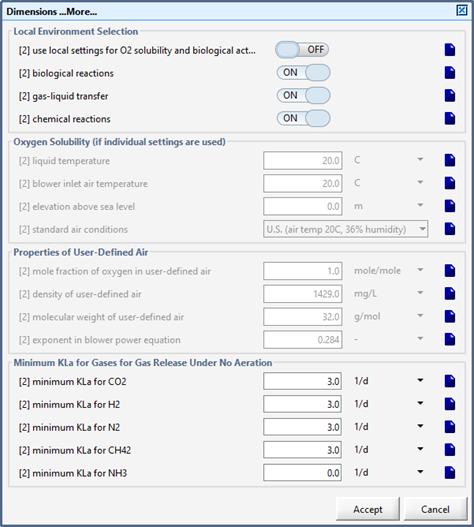
Figure 6‑5 - Physical > More... Form within an Object
Use local settings for O2 solubility and biological activity (ON – OFF): Selects whether local or global conditions are used for oxygen solubility.
Liquid temperature: Allows the user to specify the local wastewater temperature
Blower inlet air temperature: Allows user to specify the inlet air temperature for the blowers.
Elevation above sea level: Specifies the elevation above sea level.
Standard air conditions (U.S. (air temp 20°C, 36% humidity)/ European (air temp 0°C, 0% humidity/User-Defined): If the aeration method is diffused, this switch selects which standard conditions are used to calculate the standard air flow used within GPS-X and displayed as an output. If user-defined standard air is selected, the user must enter the properties of their air in the Properties of User-Defined Air sub-section. The user-defined air option provides the user with a method of specifying pure oxygen.
Mole fraction of oxygen in user-defined air: When user-defined standard air has been selected, this parameter specifies the oxygen mole fraction of the user-defined air. The default value is 1 which is consistent with pure oxygen.
Density of user-defined air: When user-defined standard air has been selected, this parameter specifies the density of the user-defined air. The default value is 1,429 mg/L which is consistent with pure oxygen.
Molecular weight of user-defined air: When user-defined standard air has been selected, this parameter specifies the molecular weight of the user-defined air. The default value is 32 g/mole, which is consistent with pure oxygen.
Exponent in blower power equation: When user-defined standard air has been selected, this parameter specifies the value of exponent K in Equation 6.28 for the user-defined air. The default value is 0.284, which is consistent with pure oxygen.
When global conditions are being used for oxygen solubility or it is necessary to change global physical constants important to aeration, the relevant physical data is accessed by selecting System > Input Parameters > Physical Environment Settings. The available parameters are shown in Figure 6‑6 and are detailed below.
Most of the parameters in this sub-section of the layout-wide physical form are duplicates of the local versions discussed earlier. The one exception is as follows:
Barometric pressure at sea level: Specifies the pressure at sea level. The default value is 101.325 kPa.
The parameters in this sub-section of the layout-wide physical form are duplicates of the local versions discussed earlier.
By clicking on the More… button in the Properties of User-Defined Air section, the user can specify the regression coefficients used in the available SOTE correlations.
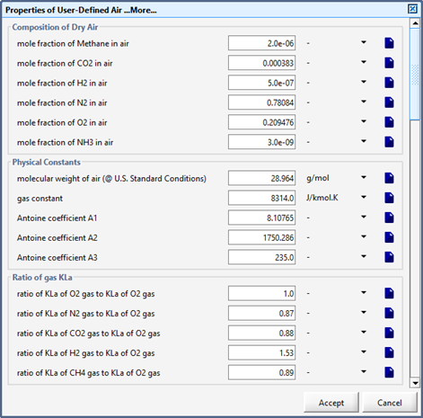
Figure 6‑6 - Physical Environment Settings (Layout-Wide Settings)
Molecular weight of air (@ U.S. Standard Conditions): Specifies the molecular weight of air at U.S. Standard Conditions which is used in Equation 6.5 to calculate the barometric pressure at the elevation and air temperature specified. GPS-X does its internal calculations in U.S. Standard Conditions.
Gas constant: Specifies the value of the universal gas constant.
Antoine coefficient A1: Coefficient A in the Antoine equation which is used to calculate the vapour pressure of water at a given water temperature.
Antoine coefficient A2: Coefficient B in the Antoine equation which is used to calculate the vapour pressure of water at a given water temperature.
Antoine coefficient A3: Coefficient C in the Antoine equation which is used to calculate the vapour pressure of water at a given water temperature.
The blower cost sub-section can be accessed by right-clicking on most biological objects and selecting Input Parameters > Operating Cost. The GPS-X form is shown in Figure 6‑7. The available parameters are described below.
Combined blower/motor efficiency: Specifies the overall efficiency of the mechanical aeration equipment (i.e. blowers, motors, coupling, and gear box). The default value is 0.7 or 70 % efficiency.
Pressure drop in inlet filters and piping to blower: Specifies the pressure drop in the inlet filters and piping to the blowers for the purposes of calculating the wire power supplied to the mechanical aeration equipment. The default value is 1 kPa.
Pressure drop in piping and diffuser downstream of blower: Specifies the pressure drop in the piping and diffusers downstream of the blowers for the purposes of calculating the wire power supplied to the mechanical aeration equipment. The default value is 7 kPa.
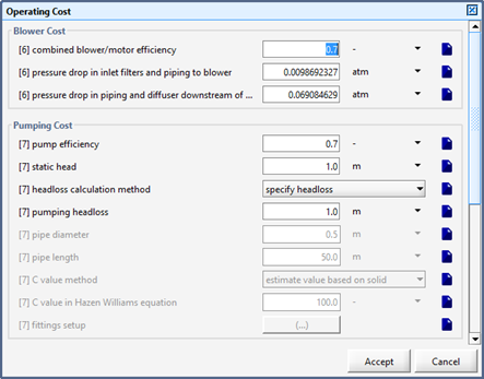
Figure 6‑7 - Blower Cost Form
The aeration output variables can be accessed by right-clicking on most biological objects and selecting Output Variables > Oxygen Transfer. For single tank objects, the same form can be accessed by right-clicking on the overflow stream. For muli-tank objects such as the plugflow tank, the total airflow, SOTR, OTR, and mechanical power can be accessed by right-clicking on the overflow stream and selecting Total Air Flow, Total Oxygen Transfer, or Total Mechanical Power.
The output
variables associated with the blower calculations can be accessed
by right-clicking on the object (single tank objects only) or the
overflow stream and selecting
Output Variables > Operating Cost.
In the Membrane Bioreactor and Completely-Mixed MBR objects the biological air and cross-flow air in the membrane tanks are tracked separately. The biological air is handled similarly as in the other objects in GPS-X with the exception that surface mechanical aeration is not an available option.
The cross-flow air is assumed to be delivered using a coarse bubble aeration system. The user can enter the following variables for the cross-flow air: air flow, alpha, and SOTE. The cross-flow air is assumed to be at the conditions specified for the biological air (i.e. Standard or Field). Unlike other objects in GPS-X, the user can specify whether the air is at standard or field conditions even if the user is not entering the biological airflow. GPS-X tracks the biological and cross-flow air separately but also calculates the total air flow, SOTR, and OTR delivered to the tank.
In the MBR objects, lower default alpha values are used to reflect the high MLSS concentrations typically found in MBRs.
This model extends the capability of the standard aeration model in activated sludge unit process models to simulate the head-loss in the air delivery model, thus simulating the dynamic changes in the blower discharge pressure. The air delivery head loss model can be used to simulate the following losses in air delivery system.
1) Air diffuser
2) Air delivery pipes and fittings
3) Control valve
In the air delivery head loss model, the required air flow rate in each biological reactors (user specified or calculated by DO controller) are used to estimate head-losses in various components of the air delivery system. To model the air delivery system, the model uses a predefined air delivery system as shown below. The model is based on the proposed model by Gray and Kestel, 2013 with some modifications.
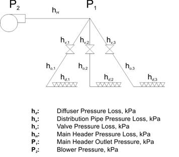
Figure 6‑8 - Predefined air delivery system
The pressure loss calculations for the diffuser, air pipe and control valve are described in following sections.
The diffuser head loss is calculated based on a diffuser head loss curve. The head loss curve is defined by the user by providing a number of points specifying air flow rate per diffuser and the expected head loss. The air flow rate per diffuser is calculated based on the air flow rate requirement and the number of diffusers in each tank set by the user in the aeration menu. The user may use available diffuser head loss curves from the aeration system supplier. The default diffuser head loss curve in model is as shown below.
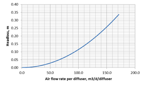
Figure 6‑9 - Default curve for diffuser head loss
User may refer to ASCE (1988) reference on Aeration for the expected diffuser head loss from different diffuser systems.
The head loss in a straight pipe is calculated using the following equation (Qasim, 1999).
Equation 6.32
![]()
Where:
![]() -
head loss, m H2O
-
head loss, m H2O
f - friction factor,-
L - length of pipe,m
D - pipe diameter, m
Qair - air flow are, m3/min
P - air supply pressure, atm
T - temperature in pipe, oK
The friction factor is calculated using the following equation:
Equation 6.33
![]()
The temperature in pipe is estimated as below:
Equation 6.34
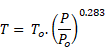
Where:
To - ambient air temperature, oK
Po - ambient barometric pressure, atm
The minor fitting losses in the ell, tees and other fittings are estimated using the pipe head loss equation as above. The user is required to estimate the equivalent length of the fittings and input it into the model (Qasim, 1999).
The user may use the following equation to find the equivalent length of the fittings.
Equation 6.35
![]()
Where:
L - Equivalent length of pipe fitting, m
C - C value for equivalent pipe length
D - Diameter of fitting, m
The C values for the fitting are typically available from the manufacturer/supplier.
The head loss in a valve is estimated based on the following equation used by Gray and Kestel, (2013).
Equation 6.36
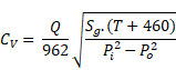
Where:
Q - air flow rate, scfm
Pi -inlet pressure, psia
Po -outlet pressure, psia
T - temperature, oK
Sg - specific gravity of air,-
CV - valve flow coefficient,
The specific gravity of air is estimated at the pressure and temperature of air in pipe as estimated for the pipe head loss. The valve flow coefficient depends on the valve position and the valve characteristics curve. The model uses linear, equal percentage, hyperbolic, exponent and square root valve characteristic curve equations to estimate the valve flow coefficient. The equations used are as below.
Linear
Equation 6.37
![]()
Equal Percentage
Equation 6.38
![]()
Hyperbolic
Equation 6.39
![]()
Exponent
Equation 6.40
![]()
Square Root
Equation 6.41
![]()
Where:
CV - valve flow coefficient, scfm/psia
CV,max - valve flow coefficient at fully open valve, scfm/psia
VP - valve position (0 – 1), -
VR - valve factor for the curve, -
m - exponent, -
For a given air flow rate in each reactor, the model estimates the head loss in diffusers, drop pipes and fittings and control valves. Based on the hydrostatic pressure and the calculated head losses, the pressure at point P1 and P2 (Figure 6‑8) are estimated. The pressure at point P1 is balanced by manipulating the valve positions. Two algorithms of Most Open Valve (MOV) and Set Point Pressure are implemented. In MOV algorithm, the valve corresponding to the maximum head loss is opened until it is open to specified maximum and then the other valves are adjusted to achieve the same pressure as estimated by the MOV. In the Set Point Pressure method, all the valves are adjusted to achieve the set point blower pressure.
A few comments about the state variables used in each of these models is required. For all the models, the symbolic name of the state variables is prefixed with either an X for particulate component, S for soluble component, or in some cases a G for gaseous component. This designation follows the IWA (Henze et al., 1987a) convention, but is somewhat arbitrary because some soluble and particulate components are colloidal and will pass through a 0.45mm filter but still be classified as part of a particulate component.For example the slowly biodegradable material, designated Xs, may include soluble and/or colloidal material. This approach greatly facilitates the model development; however it invariably introduces some error into the models. The issues of wastewater characterization are important and the modeller should refer to the papers listed with the individual models discussed below.
Most biological process models now follow a standard matrix format. An example of this format is shown in Table 6‑1.
Table 6‑1 – Example Model Matrix (Wentzel et al., 1987a)
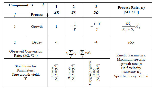
In this table, the components or state variables of the Monod-Herbert model (Herbert, 1958), designated by a variable with a subscript i, are numbered and listed across the top. Three state variables are defined (Xb, SS and So), each having its own column. Names and units for each state variable are provided in the bottom row of each of these columns. The important processes, designated pj, in the system, which result in changes in the state variables, are shown in separate rows; the actual process rate (kinetic expression or rate equation) is shown in the rightmost column of each of these rows. All the necessary kinetic parameters are defined in the lower right-hand corner of the table.
The entries within the table are the stoichiometric parameters or relations, designated vij, used in defining the net process rate for a component. These parameters define the mass relationships between components and are defined in the lower-left hand corner of the table. If a process does not directly affect a component's rate, then the table cell will be empty (the entry is assumed to be zero in this case).
The net reaction rate of a component, designated ri, is the sum of all the process rates, which cause a change in the mass of that component. The expression used to determine the net rate is listed in the table in the row labeled "Observed Conversion Rates". When the model is presented in matrix format, this equation has a simple visual interpretation. To determine the net rate of change for a component, first identify the column of the component of interest and move down that column until you find a table cell containing an entry. Multiply the table cell entry by the process rate shown in the rightmost column. The sum of these individual process rates is the net reaction rate. Do likewise for all remaining rows in the column, which contain stoichiometric parameters.
Two common stoichiometric parameters appearing in the biological models in this chapter are derived from their respective chemical equations. First is the nitrogen to oxygen stoichiometric parameter used in the denitrification equation. A value of 2.86 is used throughout the GPS-X libraries for all the biological models. This value is derived from the molecular ratios shown in the equation below:
Equation 6.42
![]()
The ratio of mass oxygen produced per mass nitrogen gas produced is 160:56 or 2.86:1. Similarly, the stoichiometric ratio of oxygen to nitrogen required for nitrification (used in many of the biological models) has a value of 4.57 which is derived from the molecular ratios shown in the equation below:
Equation 6.43
![]()
The ratio of mass of oxygen to mass of nitrogen is 64:14 or 4.57:1.
Since these stoichiometric ratios cannot change, the values are hard-coded in GPS-X without user access.
The International Association on Water Pollution Research and Control (IAWPRC) Task Group realized that due to the long solids retention times and low growth rates of the bacteria, the actual effluent substrate concentrations between different activated sludge treatment plants did not vary greatly. What were significantly different were the levels of MLSS and electron acceptor (oxygen or nitrate). Thus the focus of the Activated Sludge Model No. 1 (called asm1 in GPS-X) is the prediction of the amount and change of the solids and electron acceptor.
The Task Group considered the trade-off between model accuracy and practicality. They identified the major biological processes occurring in the system and characterized these processes with the simplest rate expressions that could be used, resembling the real reactions.
The use of switching functions was made by the Task Group since some reactions depended on the type of electron acceptor present. These functions were of the form:
Equation 6.44

At low concentrations of dissolved oxygen (SO), the parameter KOH dominates the expression and approaches a value of zero. At high values of SO, the parameter KOH would be negligible and the expression approaches unity. If the switching function was inverted, then the limits when SO were high or low are reversed. A consequence of using switching functions of this form is that they are continuous functions unlike discontinuous on/off switches which are more difficult to simulate.
In the development of activated sludge modelling, the manner in which the quantity of organic matter is measured (BOD, COD or TOC) is inconsistent. The Task Group decided to use COD since mass balances can be carried out and since it has links to the electron equivalents in the organic substrate, biomass and electron acceptor.
The organic material is categorized according to a number of characteristics. First, is the biodegradability of the material. The non-biodegradable organics pass through the system unchanged and can be further categorized according to their physical state (soluble or particulate), which is removed from the system by different pathways. The particulate material is generally removed with the waste activated sludge, while the soluble material leaves with the effluent. The biodegradable material is categorized as either readily or slowly biodegradable. The Task Group treated the former as soluble material, while the latter was treated as particulate material (this is not strictly correct, but simplifies matters). The readily biodegradable organics may be utilized for cell maintenance or growth with a transfer of electrons to the acceptors. The particulate (slowly) biodegradable substrate is hydrolyzed to readily biodegradable material, assuming no energy utilization and no corresponding use of electron acceptor.
The hydrolysis rate is usually slower than the utilization of readily biodegradable substrate so that it is the rate limiting step, if only slowly biodegradable substrate is available.
Two types of biomass are modelled:
1. heterotrophic; and
2. autotrophic
The heterotrophic biomass is generated by the growth on readily biodegradable substrate under aerobic or anoxic conditions and decays (including endogenous respiration, death, predation and lysis) under all conditions. The autotrophic biomass is generated under aerobic conditions only utilizing ammonia for energy and decays under all conditions.
The nitrogenous material is categorized according to its biodegradability and physical state. The non-biodegradable particulate material is modelled as a fraction of the non-biodegradable particulate COD, while the non-biodegradable soluble material is ignored. The biodegradable nitrogenous material is divided into ammonia (free and ionized), soluble organic and particulate organic. Particulate organic is hydrolyzed to soluble organic, while soluble organic is converted to ammonia by the heterotrophic biomass. The conversion of ammonia to nitrate by the autotrophs is assumed to take place in one step.
The Model Matrix for asm1 is found in Appendix A.
Asm2 is no longer implemented in GPS-X, in favour of using the asm2d model (see below), which corrects errors and deficiencies from the original published model.
This model (asm2d) is an implementation of the Activated Sludge Model No. 2d (Henze et al., 1998). The model structure, default values and all other model aspects follow the publication in every detail.
This model is an extension of asm1, primarily to handle biological phosphorus removal systems. The model matrix is shown with the nomenclature used in the GPS-X implementation. Users of this model should consult the reference (Henze et al., 1998) for details of this model.
The asm2d model is implemented in the CNP and CNPIP library, and the Model Matrix is found in Appendix A.
One major difference in the way this model is presented compared with the other models is seen in its matrix description. The stoichiometric coefficients for ammonia and soluble phosphorus are listed outside the table. The reason behind this is that to eliminate the organic nitrogen state variables (xnd and snd); they are now incorporated into the other soluble and particulate organic components as a fixed fraction. Similarly, a fixed fraction of phosphorus is included in the organic components.
Each of these state variables represents a spectrum of organic biodegradable material. Another state variable is used to model the other soluble organic material, which is not biodegradable (si). This material is part of the influent and can be produced during some hydrolysis processes. The soluble nitrogen components consist of 1) ammonia and ammonium (snh); and 2) nitrate and nitrite (sno). The dinitrogen gas produced (snn) is also modelled, but is considered insoluble and immediately comes out of solution. Oxygen (so) and inorganic soluble phosphorus (sp) are the other two soluble states. The inorganic soluble phosphorus is typically ortho-phosphate.
Looking at the particulate states, the model includes three types of biomass:
1. heterotrophic organisms (xbh);
2. nitrifying organisms (xba); and
3. phosphate accumulating organisms (xbp)
The phosphate accumulating organisms’ state variables do not include the internal storage products, which are separate state variables. Particulate non-biodegradable organic material is also modelled (xi). Although it is not removed from the system, it may be generated during cell decay. The two internal storage products of the phosphorus accumulating organisms are:
1. internally stored COD (xbt); and
2. poly-phosphate (xpp).
Neither of these two components is included in the mass of the phosphorus accumulating organism. The last state variable is the slowly biodegradable substrates (xs) which must undergo hydrolysis before available as a substrate. Particulate inorganic inert solids (xii) are present in the system, but do not interact with the biological model.
The processes described by this model are separated into four groups:
1. processes involving hydrolysis;
2. processes involving heterotrophs;
3. process involving autotrophs; and
4. processes involving phosphorus accumulators.
The hydrolysis processes include the aerobic, anoxic and anaerobic hydrolysis of slowly biodegradable organic material into soluble substrate (processes 1-3). The rate equations are similar for the three processes; however, the rate constants under these different environmental conditions are not well known. The hydrolysis of organic nitrogen is not explicitly included in this model. Rather, a fraction of the organic particulate material is assumed to be organic nitrogen and therefore hydrolyzes at the same rate as the organic particulate substrate.
The heterotrophic processes include the aerobic growth on two substrates (processes 4 and 5), their corresponding anoxic growth (processes 6 and 7). The fermentation of organic material under anaerobic conditions is also accounted for by process 8. This process has been identified as one requiring more research into its understanding. Since little is known about this process, a large range of kinetic parameters for this rate may be found during the modelling exercise. Process 9 models the death and lysis of the heterotrophs.
Processes 10-15 describe the phosphorus accumulating bacteria:
1. the internal storage of fermentable products (process 10);
2. the internal storage of poly-phosphate (process 11);
3. the aerobic growth of polyP bacteria (process 12); and
4. the lysis of the bacteria and their corresponding internally stored products (processes 13-15)
The final two processes in the model are the aerobic growth of the nitrifiers (process 16) and their death and lysis (process 17). The kinetic parameters of this model, like those of the mantis model, are temperature dependent. A similar Arrhenius type function is used to describe this dependency.
This model is a minor extension of the original asm2 model. It includes two additional processes to account for phosphorus accumulating organisms (PAOs) using cell internal storage products for denitrification. Whereas the asm2 model assumed PAOs to grow only under aerobic conditions, the asm2d model includes denitrifying PAOs.
The Activated Sludge Model No. 3 (Gujer et al., 1999) relates to ASM1 and corrects for some inadequacies of ASM1. The main features of the model are:
· Hydrolysis is independent of the electron donor, and occurs at the same rate under aerobic and anoxic conditions.
· Lower anoxic yield coefficients are introduced.
· Decay of biomass is modelled as endogenous respiration (vs. the “death regeneration” concept used in asm1).
· Storage of COD by heterotrophs under anoxic and aerobic conditions is modelled.
· It is possible to differentiate between anoxic and aerobic nitrifier decay rates.
· Ammonification of SND and hydrolysis of biodegradable, particulate nitrogen (XND) are omitted. Instead, a constant composition of all organic components has been assumed (constant N to COD ratio).
· Alkalinity limitation on the process rates is considered.
Figure 6‑10 shows a schematic of the processes simulated in the asm3 model.
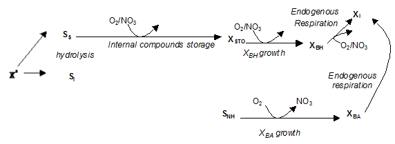
Figure 6‑10 - ASM3 Model Processes
The Model Matrix for asm3 is found in Appendix A.
The mantis model is identical to the IAWPRC Activated Sludge Model No. 1 (asm1), except for the following modifications:
· Two additional growth processes are introduced, to allow for growth of heterotrophic biomass with nitrate as a nutrient.
· Switching functions for nitrogen as a nutrient (and phosphorus, in applicable libraries) and alkalinity for growth
· Separate half-saturation coefficients for oxygen for aerobic and anoxic growth, to allow for calibration of simultaneous nitrification/denitrification.
The additional growth processes account for the observed growth of organisms during conditions of low ammonia and high nitrate. Under these conditions, the organisms can uptake nitrate as a nutrient source.
The temperature dependence of the kinetic parameters is described by an Arrhenius equation. See Appendix A for the Model matrix describing this model.
Aerobic denitrification is included in the model according to the Münch modification (Münch et al., 1996). In many cases modellers have seen nitrate levels overpredicted in their models due to the simplifications in spatial resolution (ideally mixed aeration tanks, no oxygen diffusion limitation in floc cores, etc.). The new modification, consisting of one new anoxic oxygen half-saturation coefficient makes anoxic growth rates adjustable independently from aerobic growth, and the coefficient itself is an indication of the degree of aerobic denitrification occurring within the plant modelled. The default value of the new constant is set equal to the aerobic oxygen half saturation.
Dold's general model is not implemented in GPS-X, in favour of the newgeneral model. However, a description of the general model (which makes up the basis for the newgeneral model) is presented here.
In the following sections, the general model of Dold (1990) is described. This model was derived from a combination of the asm1 model for non-polyP heterotrophic organisms and autotrophic organisms (Henze et al., 1987a, 1987b) and the Wentzel et al. (1989b) model for polyP organisms.
The general model component proposed for describing the kinetic response of the non‑polyP heterotrophic and autotrophic organism masses is based on the asm1 model (Henze et al., 1987a, 1987b), with three modifications/extensions:
1. The nitrogen source for cell synthesis
2. Conversion of soluble readily biodegradable COD to short-chain fatty acids (SCFA’s).
3. Growth of non-polyP heterotrophs on SCFA.
In reviewing the initial asm1 model version, Dold and Marais (1986) postulated that under certain circumstances, nitrate, instead of ammonia nitrogen, may serve as the nitrogen source for cell synthesis purposes. This postulate was confirmed from analysis of data collected over an extensive period, particularly in multiple series reactor configurations operated at long sludge ages and which exhibited high nitrification rates. The use of nitrate as a nitrogen source for polyP organism synthesis, when the ammonia concentration dropped to low levels, was also observed by Wentzel et al., (1989b). On the basis of this information, an additional two processes have been incorporated into the asm1 model version to give four growth processes: aerobic and anoxic growth of non-polyP heterotrophs with either ammonia or nitrate as the N source for synthesis.
In the asm1 model, readily biodegradable soluble COD is utilized by the non-polyP organisms (i.e. heterotrophs) in four possible growth modes - under aerobic or anoxic conditions with either ammonia or nitrate as the nitrogen source for synthesis purposes. For biologically-enhanced phosphorus removal (BEPR) systems it is necessary to distinguish between "complex" and SCFA readily biodegradable COD; therefore, it is necessary to duplicate the four growth processes in the asm1 model to account for possible growth on the two components of the readily biodegradable COD for the mixed culture system. With regard to growth on SCFA it is likely that only one of the four processes would be of consequence - anoxic growth with ammonia as the N source. This is because SCFAs are removed in the unaerated zones at the "front end" of the continuous flow systems and do not enter the aerobic zones in appreciable concentrations. However, for completeness all four growth processes in the asm1 model (for "complex" COD) were duplicated in the general model for growth of non-polyP organisms with SCFA as substrate. The same kinetic formulations and stoichiometry for growth on "complex" readily biodegradable COD and SCFA have been used.
The general model component proposed for describing the kinetic response of the polyP heterotrophic organism mass is based on the enhanced culture model of Wentzel et al. (1989b), with one additional process for anoxic growth of polyP organisms described by Dold (1990) (and the one additional stoichiometric constant, fup, for anoxic growth). It should be noted that the phenomenon of accumulation of un-biodegradable soluble COD from endogenous processes in the enhanced cultures also received attention. Wentzel et al. (1989a) suggested that this material would be used as a substrate source by non-polyP organisms in mixed culture systems.
While this is likely, no change was made to the model in this respect because the amount of generation in the mixed culture systems is small.
The values of the kinetic parameters, as with the asm1 model, are those for 20°C.
The general model is no longer available in GPS-X, in favour of using the newgeneral model (see below), which corrects deficiencies of the general model.
The newgeneral model is based on the general model with significant changes to account for so-called 'COD losses' that have been reported in nutrient removal systems.
Some key features of the newgeneral model include:
· ‘COD’ loss yields
· Hydrolysis efficiency factors
· Heterotrophic yield coefficients for different electron acceptor conditions.
The modelling of BNR activated sludge systems has identified mass balance problems in some facilities. That is, several experimental and full-scale evaluations of BNR facilities have revealed imbalances between what is going into the plant and what is going out (i.e. less COD is going out than going in, hence the COD 'loss'). Both from a theoretical and modelling point of view this causes some problems, and there is no world-wide accepted explanation for these imbalances. Nevertheless, these discrepancies must be modelled. To account for these mass balance problems (referred to as anaerobic stabilization or COD losses), four COD loss terms are included in the newgeneral model. These include:
· Hydrolysis efficiency factor (anoxic)
· Hydrolysis efficiency factor (anaerobic)
· Fermentation volatile fatty acid (VFA) yield.
· PolyP PHB yield on sequestration of VFAs.
The newgeneral model has proven itself to be a reliable predictive tool for the BNR process. Nevertheless, users should be aware that the newgeneral model in its default condition does not result in a COD balance across the system. To eliminate COD losses (and thus force a COD balance across a newgeneral -based layout) each of these stoichiometric loss terms should be set to 1.0.
Included in newgeneral are two new heterotrophic yield terms to account for differences in yield under varying electron acceptor conditions. Where the general model assumed the same yield irrespective of the electron acceptor, newgeneral differentiates the yield depending on the presence of oxygen and nitrate. The added stoichiometric terms include:
· Yield (anoxic)
· Yield (anaerobic)
In total, two state variables and eight processes have been added to the general model.
· Non-releasable polyphosphate (XPP)
· Soluble inorganic nitrogen (SNI)
· Anoxic hydrolysis of stored/enmeshed COD
· Anaerobic hydrolysis of stored/enmeshed COD
· XPP lysis on aerobic decay
· XPP lysis on anaerobic decay
· Anoxic decay of PolyP organisms
· XPPR lysis on anoxic decay
· XPP lysis on anoxic decay
· XBT lysis on anoxic decay
As evidence exists that not all polyphosphate is releasable, a new state variable to represent non-releasable polyphosphate was incorporated. The uptake of phosphorus (both aerobically and anoxically) in newgeneral results in the storage of both releasable and non-releasable polyphosphate. The partitioning of the storage is stoichiometrically determined based on the total phosphorus taken up.
In the general model decay of PolyP organisms was modelled as an aerobic or anaerobic process. The newgeneral model includes anoxic decay of XBP to those processes. This results in the anoxic lysis of XBT and XPPR modelled in a similar way to the aerobic lysis of these variables in the general model. To account for the lysis of XPP, newgeneral includes three new processes: one for aerobic lysis, one for anoxic lysis and one for anaerobic lysis.
The hydrolysis of particulate COD to soluble material suitable for growth is a critical step in the COD cycle. The general model modelled hydrolysis as an aerobic process only, butnewgeneralincludes hydrolysis under anoxic and anaerobic conditions and uses these processes as a sink for COD 'loss.
Whereas the fermentation of SS to SLF was a non-growth related process in the general model, in newgeneral, this process is associated with the growth of heterotrophic organisms and hence, a portion of the fermented COD winds up as new biomass; however, equally important is the stoichiometry of this process because, like hydrolysis, this process includes a COD 'loss' component.
The Model Matrix for the newgeneral model is found in Appendix A.
A new comprehensive model incorporating the most commonly observed biological, physical, and chemical processes in wastewater treatment plants was developed and implemented in GPS-X. MANTIS2 is the outcome of Hydromantis’ commitment to provide state of the art models to its clients through research and development. The MANTIS2 model incorporates a large amount of information which has become available in technical literature in the last decade. The motivation behind the development of a comprehensive model arises from the fact that after the publications of ASM2d and ADM1, there has been growing interest in extending the capabilities of models to incorporate the side stream treatment processes like struvite precipitation, nitrification-anammox for nitrogen removal, and other precipitation processes. Although state variable interfaces between ASM2d and ADM1 are well defined, the state variable mapping between two models present practical challenges in model implementation and limits the versatility in modelling.
The key features of the MANTIS2 model are:
· Carbon, Nitrogen, and Phosphorus removal with integrated anaerobic digestion processes.
· Mass balance for COD, C, N, P, Ca, Mg, K, and charge
· 48 state variables (21 soluble + 27 particulate)
· 56 processes
· Two-step nitrification using AOB, NOB
· Two-step denitrification
· Methanol degradation process with methylotroph biomass
· ANAMMOX process
· Anaerobic digestion processes with gas phase modelling for N2, CO2, H2, and CH4
· pH and alkalinity estimation in both liquid and solid train
· Precipitation of MgNH4PO4. 6H2O, CaCO3, MgHPO4. 3H2O, CaPO4, AlPO4, FePO4, Al(OH)3 and Fe(OH)3
· Unified composite variable calculation
The MANTIS2 model is is implemented in MANTIS2LIB. The MANTIS2 model allows estimation of pH in both the liquid and solid train, therefore it is possible in MANTIS2 to use additional influent objects like acid feed, alkali feed to estimate the chemical required for pH adjustment.
The basic structure of the comprehensive MANTIS2 model is based on the following published models:
1. ASM2d – basic reactions for biological carbon, nitrogen, and phosphorus removal
2. UCTADM1 – Anaerobic digestion processes
3. Musvoto Model – Inorganic precipitation processes
In addition to the above, reference is made to other accepted models (i.e. newgeneral model, ADM1 and UCTCN and MANTIS) in formulating the model structure and finalizing the default stoichiometry and kinetics of model parameters. The modelling approaches for two-step nitrification, two-step denitrification, denitrification on methanol and ANNAMOX are adopted from recent research studies.
A complete description of the state variables in MANTIS2 model is located in the Comprehensive Model Library (MANTIS2LIB) section of 0.
The soluble states in the model can be classified into four categories: Soluble inert organic; Soluble biodegradable organics; Soluble inorganic ions; and Dissolved gases. The states in each category are described in following sections.
Soluble Inert Organics
1. Soluble inert organics (si)
The state represents the inert organics in the wastewater. The soluble inert organics are not degraded in the wastewater treatment processes. MANTIS2 model considers the generation of soluble inert organic during the hydrolysis of slowly biodegradable substrate. By default, the fraction of soluble inert organic production is set to zero. In the anaerobic digestion process, the fraction may be set to a non-zero value to calibrate the soluble inert COD from the digesters.
Soluble Biodegradable Organics
1. acetate (sac)
2. propionate (spro)
3. methanol (smet)
4. fermentable substrate (ss)
5. colloidal substrate (scol)
The state of fermented substrate (slf) in ASM2D is split into two states of acetate (sac) and propionate (spro). The inclusion of an additional state of spro is required as it is one of the important intermediate products in anaerobic digestion.
The additional state of methanol (smet) is added to the model. It is now well accepted that the single carbon methanol is degraded by special microorganism which have different kinetics than the ordinary heterotrophic organism. This additional state is helpful to track the degradation of methanol based on the degradation kinetics of methylotrophic biomass.
Although there is no well accepted definition of the state of colloidal substrate in wastewater, for the purpose of modelling, it is assumed that this fraction represents the portion of the substrate COD which lies in the size range of 0.45 micrometers to 1.2 micrometers. These are typically macromolecules which require hydrolysis before oxidation. This fraction of COD is assumed to behave differently in different unit processes for example the colloidal COD will behave:
· as soluble in solid liquid separation in settlers
· as particulate in biological degradation
· as particulate or soluble in membrane separation
Soluble Inorganic
In addition to the soluble organic states, the MANTIS2 model considers inorganic states of soluble inorganic carbon (stic), soluble nitrite-N (snoi), soluble nitrate-N (snoa), soluble Ammonia-N (snh), soluble Organic nitrogen (snd), soluble ortho-P (sp), dissolved calcium (sca), dissolved (smg), dissolved potassium (spot), dissolved anion (sana) and dissolved cation (scat). These inorganic states are chosen so as to appropriately describe the N and P transformation, inorganic precipitation and pH changes across the various unit processes in wastewater treatment plant.
The soluble inorganic carbon, stic, represents the sum of carbon in all the ionic species in the carbonic acid system i.e. H2CO3, HCO3-, CO32-. In previous models like ASM2D and New General, the alkalinity (salk) is used to express the buffer capacity in the wastewater. In MANTIS2, soluble inorganic carbon is used instead of alkalinity as the state variable as it is a conserved quantity. The alkalinity in the model is estimated by considering the soluble inorganic carbon and the estimated pH of the system.
Two oxidized form of soluble nitrogen, (i.e. soluble nitrite and nitrate) are considered in the model. This choice is necessary to model the two step nitrification process.
The additional inorganic states like soluble calcium (sca), soluble magnesium (smg) are introduced to model the key precipitation reaction involving these ionic species. The state variable of soluble potassium (spot) is included to model the uptake and release of potassium during polyphosphate formation and degradation. The dissolved anion (sana) and cation (scat) represent all other strong anion and cation in the wastewater. These states are used in formulating the charge balance equation for estimating the pH in the wastewater.
Soluble Gases
In addition to soluble oxygen (so), MANTIS2 includes soluble gases states for nitrogen (sn2), methane (sch4) and hydrogen (sh2). The soluble CO2 is estimated by the pH and the stic concentration in the wastewater. The soluble oxygen plays an important role in the aerobic biological systems. The other gases are more relevant in the anaerobic digestion and fermentation processes. For each soluble gas, gas-liquid transfer equation are used to model the dissolution/stripping of the gas in the unit processes.
The particulate states in the model are classified into four categories of Particulate Inert Organics, Particulate Organic Substrate/Storage, Active Biomass and Particulate Inorganic.
Particulate Inert Organics
The model includes two states of Inert Organic Particulate (xi) and Unbiodegradable Organic Matter from cell decay (xu) in the model. The inert organic particulate is the inert organics fraction that is contributed by the influent wastewater. Having two states for inert organic compounds makes it easier to differentiate between the amount of inert organics accumulated from the wastewater and the amount that is produced by cell decay in the system.
Particulate Organic Substrate/Storage
MANTIS2 provides one particulate Organic Substrate (xs) and one organic storage compound for intracellular PHA (xbt). These states are equivalent to the states in ASM2D and New General Models.
Active Biomass
Several biomass states are added in MANTIS2. To model the two step nitrification process, two autotrophic biomass Ammonia Oxidizer (xbai) and Nitrite Oxidizer (xbaa) are considered. Methylotrophic biomass (xbmet) is included to model the biodegradation of methanol. The fermentive biomass (xbf), Acetogen (xbpro), acetate methanogens (xbacm) and hydrogen methanogens (xbh2m) are included to model the anaerobic transformation in anaerobic digestion.
Particulate Inorganic
The particulate inorganic states include the model precipitates like aluminum hydroxide, aluminum phosphate, iron hydroxide, iron phosphate, calcium carbonate, calcium phosphate, magnesium hydrogen phosphate, magnesium carbonate, and ammonium magnesium phosphate (struvite). In addition to these precipitates, particulate inert inorganic is used as a composite state for the unidentified inorganic in the wastewater. The N and P components associated with the slowly biodegradable organics are included as nitrogen in slowly deg. organics and phosphorous in slowly deg. organics. The inorganic poly-phosphate accumulated in PAO is also included as a state.
MANTIS2 uses a well-defined stoichiometry for each state variable to estimate the composite variables. The state variables and their relationships to the composite variables are shown in the Composite Variables in MANTIS2LIB section of 0, GPS-X Composite Variable Calculations.
The processes included in the MANTIS2 model are described below:
Adsorption/Enmeshment
1. Adsorption of colloidal COD: The colloidal COD (scol) is considered to first adsorb on the heterotrophic biomass. The adsorbed colloidal COD then becomes a part of slowly biodegradable COD (xs) and requires hydrolyses before it become available for bacterial metabolism. As both the ordinary heterotrophic organism and fermentative organism are considered to participate in the hydrolysis process, the rate of adsorption is defined with respect to the sum of the concentration of two organisms. The adsorption rate is first order to the colloidal COD. A rate inhibition term is added to reduce the rate of adsorption as the ratio of slowly biodegradable COD to adsorbing biomass increases.
Processes mediated by heterotrophic organisms
2. Aerobic hydrolysis: The heterotrophic microorganisms are considered to participate in the hydrolysis of slowly biodegradable substrate XS resulting in production of soluble fermentable substrate (ss). Surface limited hydrolysis kinetics similar to that used in ASM1 and ASM2d is used. Both the ordinary heterotrophic organism and fermentative organism are considered to participate in the hydrolysis process
3. Anoxic hydrolysis: This hydrolysis process is active under anoxic conditions. The oxygen saturation term in aerobic hydrolysis rate expression is replaced with an oxygen inhibition term. A NOX (NO2-N+NO3-N) saturation term is added to the rate expression. The specific hydrolysis rate is reduced by anoxic hydrolysis reduction factor (ηnox).
4. Anaerobic hydrolysis: This hydrolysis process is active only under anaerobic conditions. The rate expression contains oxygen and NOX inhibition terms. The specific hydrolysis rate is reduced by anaerobic hydrolysis reduction factor (ηanaer).
5. Ammonification: The ammonification process converts soluble organic nitrogen to ammonia nitrogen. Both the ordinary heterotrophic organism and fermentative organism are considered to participate in the ammonification process. The kinetics of ammonification is similar to that provided in ASM1.
6. Growth on fermentable substrate (ss) using O2 as electron acceptor: The process of heterotrophic growth takes place under aerobic conditions. The reaction rate for this process is formulated considering the concept of multi substrate kinetics outlined in ASM2d model. The growth rate is considered proportional to the ratio of fermentable substrate to total soluble substrate (ss+sac+spro) available to heterotrophic biomass. The main difference in the growth stoichiometry of different biomass is the uptake of N and P, Ca, Mg, K, anion and cation during the biomass growth. In this implementation, it is assumed that concentration of Ca, Mg and K is non-limiting during growth. If required, the saturation terms for each micronutrient can be added easily in the model equations. The growth kinetics does not use the alkalinity saturation function as it is planned to add a pH inhibition term in the growth kinetics at a later date.
7. Growth on acetate (sac) using O2 as electron acceptor: The process of aerobic heterotrophic growth on acetate is similar to the process #6, except that the growth rate is proportional to the ratio of acetate concentration to the total soluble substrate (ss+sac+spro) available to heterotrophic biomass.
8. Growth on propionate (spro) using O2 as electron acceptor: The process of aerobic heterotrophic growth on acetate is similar to the process #6, except that the growth rate is proportional to the ratio of propionate concentration to the total soluble substrate (ss+sac+spro) available to heterotrophic biomass.
9. Growth on fermentable substrate (ss) using NO3 as electron acceptor: This process of heterotrophic growth takes place in the presence of NO3-N. The stoichiometry of this process is developed by considering partial reduction of NO3-N to NO2-N. The rate expression for the process uses an inhibition term for oxygen and a saturation term for the NO3-N. The growth rate is also considered proportional to the ratio of fermentable substrate to total soluble substrate (ss+sac+spro) available to heterotrophic biomass. The reaction rate expression also reduces the amount of heterotrophic biomass by the fraction of NO3-N to total NOX nitrogen available in the system. It is assumed that when the heterotrophic biomass is converting NO3-N to NO2-N, it is not participating in the conversion of NO2-N to N2 gas.
10. Growth on acetate (sac) using NO3 as electron acceptor: The process of heterotrophic growth on acetate using NO3-N is similar to the process #9, except that the growth rate is proportional to the ratio of acetate concentration to the total soluble substrate (ss+sac+spro) available to heterotrophic biomass.
11. Growth on propionate (spro) using NO3 as electron acceptor: The process of heterotrophic growth on acetate using NO3-N is similar to the process #9, except that the growth rate is proportional to the ratio of propionate concentration to the total soluble substrate (ss+sac+spro) available to heterotrophic biomass.
12. Growth on fermentable substrate (ss) using NO2 as electron acceptor: This process of heterotrophic growth takes place in the presence of NO2-N. The stoichiometry of this process is developed by considering reduction of NO2-N to N2. The rate expression for the process uses an inhibition term for oxygen and a saturation term for the NO2-N. The growth rate is also considered proportional to the ratio of fermentable substrate to total soluble substrate (ss+sac+spro) available to heterotrophic biomass. The reaction rate expression also reduces the amount of heterotrophic biomass by the fraction of NO2-N to total NOX nitrogen available in the system. It is assumed that when the heterotrophic biomass is converting NO2-N to N2, it is not participating in the conversion of NO3-N to NO2-N gas.
13. Growth on acetate (sac) using NO2 as electron acceptor: The process of heterotrophic growth on acetate using NO2-N is similar to the process #12, except that the growth rate is proportional to the ratio of acetate concentration to the total soluble substrate (ss+sac+spro) available to heterotrophic biomass.
14. Growth on propionate (spro) using NO2 as electron acceptor: The process of heterotrophic growth on acetate using NO2-N is similar to the process #12 except that the growth rate is proportional to the ratio of propionate concentration to the total soluble substrate (ss+sac+spro) available to heterotrophic biomass.
15. Decay of heterotrophs: The process rate of heterotrophic decay is modeled similar to that in ASM2d model. The main difference in the stoichiometry of decay reaction is the production of N, P, Ca, Mg, K, anion and cation according to the biomass composition
Processes mediated by autotrophic organisms
The model considers two-step conversion of NH3-N to NO3-N. The two steps are mediated by ammonia oxidizer and nitrite oxidizer sequentially.
16. Growth of ammonia oxidizer: The process of growth of ammonia oxidizer oxidizes NH3-N to NO2-N in the presence of oxygen. The reaction rate uses ammonia and oxygen saturation terms. The stoichiometry of the process is developed based on the conversion of NH3-N to NO2-N.
17. Growth of nitrite oxidizer: The process of growth of ammonia oxidizer oxidizes NO2-N to NO3-N in the presence of oxygen. The reaction rate uses NO2-N and oxygen saturation terms. The stoichiometry of the process is developed based on the conversion of NO2-N to NO3-N.
18. Decay of ammonia oxidizer: The process rate of ammonia oxidizer decay is modelled similar to that in the ASM2d model.
19. Decay of nitrite oxidizer: The process rate of nitrite oxidizer decay is modelled similar to that in the ASM2d model.
Processes mediated by phosphate accumulating organisms (PAO)
The processes mediated by PAO are based on the ASM2D model. Three new processes describing the storage of PHA on propionate, growth of PAO on PHA using NO2 as electron acceptor and anoxic storage of XPP using NO2 are added to the processes mediated by PAO.
20. Storage of PHA by PAO using acetate: The rate expression for PHA storage by PAO using acetate as used in ASM2d is modified to include the effect of propionate, another VFA used by PAO. The rate expression is modified by assuming that PAO can utilize acetate and propionate simultaneous in proportion to the availability of each substrate
21. Storage of PHA by PAO using propionate: This is a new process and describes the storage of PHA by PAO using propionate. The kinetics and stoichiometry of the process is based on concepts used in describing process #20.
22. Growth of PAO on PHA using O2 as electron acceptor: The stoichiometry and rate expression for this process is the same as ASM2d.
23. Storage of XPP on PHA using O2 as electron acceptor: The stoichiometry and rate expression for this process is the same as ASM2d.
24. Growth of PAO on PHA using NO3 as electron acceptor: This process of PAO growth takes place in the presence of NO3-N. The stoichiometry of this process is developed by considering partial reduction of NO3-N to NO2-N. The rate expression for the process uses an inhibition term for oxygen and a saturation term for the NO3-N. The reaction rate expression also reduces the amount of PAO biomass by the fraction of NO3-N to total NOX nitrogen available in the system. It is assumed that when the PAO biomass is converting NO3-N to NO2-N, it is not participating in the conversion of NO2-N to N2 gas.
25. Storage of XPP on PHA using NO3 as electron acceptor: In this process the storage of poly-phosphate takes place while the stored PHA compounds are oxidised using NO3-N as an electron acceptor. Only partial reduction of NO3-N to NO2-N is considered in process stoichiometry formulation. Similar to the process #24, a reduction factor equal to the ratio of NO3-N to NOX-N concentration is applied to account for fraction of total biomass mediating this process.
26. Growth of PAO on PHA using NO2 as electron acceptor: This process of PAO growth takes place in the presence of NO2-N. The stoichiometry of this process is developed by considering partial reduction of NO2-N to N2-N. The rate expression for the process uses an inhibition term for oxygen and a saturation term for the NO2-N. The reaction rate expression also reduces the amount of PAO biomass by the fraction of NO2-N to total NOX nitrogen available in the system. It is assumed that when the PAO biomass is converting NO2-N to N2-N, it is not participating in the conversion of NO3-N to NO2-N.
27. Storage of XPP on PHA using NO2 as electron acceptor: In this process the storage of poly-phosphate takes place while the stored PHA compounds are oxidised using NO2-N as an electron acceptor. The conversion of NO2-N to N2 is considered in process stoichiometry formulation. Similar to the process #26, a reduction factor equal to the ratio of NO2-N to NOX –N concentration is applied to account for fraction of total biomass mediating this process.
28. Decay of PAO: The stoichiometry and rate expression for this process is same as ASM2d, except that alkalinity saturation term is not used.
29. XPP lysis: The stoichiometry and rate expression for this process is same as ASM2d, except that alkalinity saturation term is not used.
30. PHA lysis: The stoichiometry and rate expression for this process is same as ASM2d, except that alkalinity saturation term is not used.
Processes mediated by methylotrophs
A single population of methylotrophs, which degrades methanol, a single carbon substrate is incorporated in the model. Four reaction processes are considered for this biomass.
31. Growth of methylotrophs on methanol using O2 as electron acceptor: The stoichiometry and kinetics of the process is developed using the principles of heterotrophic growth. The rate expression for growth of methylotrophs includes oxygen saturation and a methanol saturation term. The biomass yield on methanol is reported to be much lower than other carbon sources. Therefore, a different yield coefficient is used in the process stoichiometry.
32. Growth of methylotrophs on methanol using NO3 as electron acceptor: The methylotrophs can use NO3-N as terminal electron acceptor to oxidize methanol. The stoichiometry of this process is developed by considering partial reduction of NO3-N to NO2-N. The rate expression for the process uses an inhibition term for oxygen and a saturation term for the NO3-N. The reaction rate expression also reduces the amount of biomass mediating the reaction by the fraction of NO3-N to total NOX nitrogen available in the system. It is assumed that when the methylotroph biomass is converting NO3-N to NO2-N, it is not participating in the conversion of NO2-N to N2 gas.
33. Growth of methylotrophs on methanol using NO2 as electron acceptor: This represents the second step of denitrification. The stoichiometry of this process is developed by considering partial reduction of NO2-N to N2-N. The rate expression for the process uses an inhibition term for oxygen and a saturation term for the NO2-N. The reaction rate expression also reduces the amount of biomass mediating the reaction by the fraction of NO2-N to total NOX nitrogen available in the system. It is assumed that when the methylotroph biomass is converting NO2-N to N2-N, it is not participating in the conversion of NO3-N to NO2-N.
34. Decay of methylotrophs: Decay of methylotrophs is modelled using first order reaction rate, with respect to the biomass concentration.
Processes mediated by Anaerobic Microorganisms
The MANTIS2 model includes processes mediated by anaerobic microorganisms. These processes present the key transformations observed in strict anaerobic environment like anaerobic digester and other modifications of anaerobic treatment technology. These processes are adapted from the anaerobic digestion model developed at University of Cape Town (UCTADM1). The process rate and stoichiometry was converted from molar units to COD units. The process stoichiometry was also modified to include the mass balances for phosphorus, Ca, Mg, K, cation and anion species. The scheme of anaerobic biodegradation assumes that the anaerobic biomass decay takes place according to the decay processes listed above. The slowly degradable substrate is then hydrolyzed anaerobically according to process 4. The resulting soluble fermentable substrate is then converted to CH4 and H2 by the processes described below.
35. Growth of fermentive bacteria at low H2: This process models the fermentation by acidogens under low H2 partial pressure. The process stoichiometry is developed based on a conversion of model fermentable substrate (glucose) to acetic acid, H2 and CO2. The kinetic expression for the process uses a H2 inhibition term to reduce the reaction rate as the partial pressure of H2 increases.
36. Growth of fermentive bacteria at high H2: This process models the fermentation by acidogens under high H2 partial pressure. The process stoichiometry is developed based on a conversion of model fermentable substrate (glucose) to acetic acid, propionic acid, H2 and CO2. The kinetic expression for the process uses a H2 saturation term to account for increased rate at higher partial pressure of H2
37. Decay of fermentive biomass: The stoichiometry and kinetic expression for the decay process of fermentative biomass is based on the same principles as for other biomass types.
38. Growth of acetogens on propionate: This process (Acetogenesis) is the process whereby the acetogens convert propionic acid under low hydrogen partial pressure. The kinetic rate expression for the process includes a H2 inhibition term and a propionic acid saturation term.
39. Decay of acetogens: The stoichiometry and kinetic expression for the decay process of fermentative biomass is based on the same principles as for other biomass types.
40. Growth of hydrogenotrophic methanogens: In this process hydrogenotrophic methanogens grow by converting H2 and CO2 to CH4. The stoichiometry of the process is based on the chemical reaction describing this process. The kinetic expression for the process uses a hydrogen saturation term.
41. Decay of hydrogenotrophic methanogens: The stoichiometry and kinetic expression for the decay process of fermentative biomass is based on the same principles as for other biomass types.
42. Growth of Acetoclastic methonegens: In this process the the acetic acid is converted to methane and CO2 by acetoclastic methanogens. The kinetic expression of the process includes an acetate saturation term.
43. Decay of acetoclastic methanogens: The stoichiometry and kinetic expression for the decay process of fermentative biomass is based on the same principles as for other biomass types.
Processes mediated by anaerobic autotrophic microorganisms
A new type of anaerobic autotrophic biomass type is included in MANTIS2 to perform anaerobic ammonium oxidation (ANAMMOX) process. The process stoichiometry is described in Strous et al. (1998) as below.
1NH4+ + 1.32 NO2- + 0.066 HCO3- + 0.13 H+ à 1.02 N2 + 0.26 NO3- + 0.066 CH2O0.5N0.15 +2.03 H2O
According to the above reaction, a mole of ammonia-N is oxidized to 1.02 mole of N2 using 1.32 mole of nitrite-N. The reaction also produces 0.26 mole of nitrate-N and leads to growth of autotrophic biomass.
To model this process, two processes are added in MANTIS2.
44. Growth of anammox microorganism: The stoichiometry factors to express the yield of biomass, NO2-N consumption and N2 and NO3- are expressed in terms of per unit NH4+-N oxidized. The reaction rate expression uses an oxygen inhibition function and NO2-N and NH3-N saturation functions. Total (ionized + non-ionized) concentration of both substrates is used in the kinetic expression.
45. Decay of anammox microorganism: Decay of anammox microorganisms is modelled using first order reaction rate with respect to the biomass concentration.
Chemical precipitation processes
The precipitation reactions in MANTSI2 are adapted from Musvoto et al. 2000 with some modifications. In addition to the processes of precipitation of AlPO4 and FePO4 which are included in ASM2d, five commonly observed precipitation processes in wastewater treatment are included in the model. The key differences from Musvoto et al. 2000 are: 1) the effect of ion-pair is neglected in the calculations; 2) the kinetic rate equations use the approach suggested in ASM2d with a few modification and 3) the mole based stoichiometry is replaced with mass based stoichiometry for maintaining model consistency. The kinetic expression for the precipitation reactions uses the concentration of participating ions, rate of precipitation and solubility product of the precipitate. The kinetic rate expression is formulated such that the precipitation and dissolution reactions can be modeled by a single equation.
46. Precipitation/dissolution of CaCO3: CaCO3 is assumed to precipitate as calcite. The calcite precipitation is assumed to take place in the presence of Ca2+ and CO32- ions in the solution. The concentration of CO32- is estimated by using the soluble inorganic carbon and the pH of the system.
47. Precipitation/dissolution of MgNH4PO4.6H2O (struvite): Struvite is the most commonly observed precipitate in the digester supernatant. The precipitation of struvite takes place if the Mg2+, NH4+ and PO43- species are present in the solution. The concentrations of NH4+ and PO43- are estimated based on the solution pH.
48. Precipitation/dissolution of MgHPO4.3H2O (newberyite): This is another precipitate of magnesium with phosphate which is normally observed at lower pH. For this precipitate, Mg2+ and HPO42- ionic species are required. The concentration of HPO42- ion is estimated based on pH of the solution.
49. Precipitation/dissolution of Ca3(PO4)2 (ACP): As the numbers of water molecules associated with the precipitate are variable, an anhydrous form is considered in expressing the mass concentration of the precipitate. It is indicated that this is probably the least stable precipitate among the possible precipitates and transforms into more stable forms with time. The Ca2+ ion and PO43- species are required in precipitation process.
50. Precipitation/dissolution of MgCO3: MgCO3 (magnesite) is another precipitate of magnesium that is included in the model. The precipitation reaction requires Mg2+ and CO32- ionic species for its formation.
51. Precipitation/dissolution of AlPO4: The precipitation of AlPO4 is required to model the metal precipitation of phosphorous in the plant. The stoichiometry of the process is similar to ASM2d; however, the kinetic expression is modified to include the solubility product of the precipitate.
52. Precipitation/dissolution of FePO4: The precipitation of FePO4 is required to model the metal precipitation of phosphorous in the plant. The stoichiometry of the process is similar to ASM2d; however, the kinetic expression is modified to include the solubility product of the precipitate.
Gas liquid transfer processes
Similar to the gas liquid transfer of oxygen, four additional processes as below are added in the model. The gas-liquid transfer is modeled using a mass transfer constant (KLa) and the gas saturation concentration at the given temperature and pressure. The mass transfer constant for each gas can be correlated to the oxygen mass transfer using gas diffusivities. For simplification, fractional factors are applied to the mass transfer constant of oxygen to obtain respective mass transfer constant.
53. Gas liquid transfer of CO2: Process describes the stripping/absorption of CO2 from/to the liquid. Since the concentration of CO2 in liquid depends on the pH, this process is very sensitive to the pH of the solution.
54. Gas-liquid transfer of N2: Process describes the stripping/absorption of N2 from/to the liquid.
55. Gas-liquid transfer of CH4: Process describes the stripping/absorption of CH4 from/to the liquid.
56. Gas-liquid transfer of H2: Process describes the stripping/absorption of H2 from/to the liquid.
In the MANTIS2 model, the pH is estimated in all the unit processes. The dissociation reactions for acid and bases are much faster than the other processes used in the model, therefore, algebraic form of equations are chosen over the differential form for expressing acid/base dissociation reactions. The pH in each unit process is estimated by solving a set of algebraic equations which include a charge balance equation along with the equilibrium equations for each ionic species. Although temperature dependency of the dissociation constant is considered in the model, ionic activity corrections are not applied in the equations. For a typical wastewater, the ionic activity correction may not be important, but at higher ionic concentrations the model pH values should be used with appropriate caution.
The MANTIS2 model uses the dissociation equations for: carbonic acid (diprotonic), phosphoric acid (triprotonic), ammonium (monoprotonic), acetic acid (monoprotonic), propionic acid (monoprotonic), nitrous acid (monoprotonic). The charge balance equation to solve for [H+] concentration is prepared using the ionized species of weak acid/base and strong anions (NO3-, sana) and strong cations (Ca2+, Mg2+, K+, scat).
The pre-fermentation model implemented in GPS-X is based on the Munch et al. model (1999), which is a mechanistic model aiming at describing the effect of design and operating parameters on the rate of VFAs production. The pre-fermenter model is found in the CSTR object only.
A general reaction pathway is shown in Figure 6‑11.
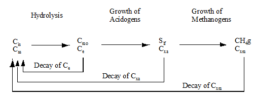
Figure 6‑11 - General Reaction Pathway
The state variables in the prefermenter model are as follows:
· Cis: insoluble substrate (not passing through a 0.45 mm filter) such as cellulose, fats, insoluble proteins (mg COD/L).
· Css: soluble, high molecular weight substrate, such as soluble carbohydrates (starch), and soluble proteins (globular) (mg COD/L).
· Cmo: monomer species such as glucose, long-chain fatty acids, amino acids (mg COD/L).
· Slf: volatile fatty acids (mg COD/L).
· Ce: hydrolytic enzymes which act as a catalyst to hydrolyse insoluble substrate, soluble high-molecular-weight substrate and proteins (mg COD/L).
· Cxa: acidogenic bacteria which utilize monomers (Cmo) as their substrate (mg COD/L).
· Cxm: methanogenic bacteria, which utilize volatile fatty acids (VFAs) as their substrate then transforming it into methane gas (mg COD/L).
· Cprot: organic nitrogen contained in particulate proteins which is converted into ammonia nitrogen in the ammonification process as particulate proteins are hydrolysed. It is also produced from the decay of bacteria cells (mg N/L).
· Snh: ammonia nitrogen (mg N/L).
· CH4,g: methane gas.
The stoichiometric parameters to be specified in the influent section are used to calculate the concentration of soluble, high molecular weight substrate (Cis) from the influent readily biodegradable substrate (ss) and the concentration of methanogenic biomass (Cxm) from the influent slowly biodegradable substrate (Xs):
· fss: fraction of soluble high molecular weight substrate (Cis) in the influent readily biodegradable substrate (ss).
· fxm: fraction of methanogenic biomass (Cxm) in the influent slowly biodegradable substrate (Xs).
· fm: conversion factor from COD to cubic meters for methane production (m3 CH4/g COD).
The stoichiometric parameters specified in the “hydrolysis”, “acidogens” and “methanogens” sections are the following yield coefficients:
· Ye: Yield for hydrolytic enzymes on insoluble or soluble substrate (Ce/Css).
· Ya: yield for acidogens on monomers species (Cxa/Cmo).
· Ym: Yield for methanogens on volatile fatty acids (Cxm/Slf).
The model kinetic parameters are:
· khis: hydrolysis rate constant for insoluble substrate (g COD/m3.d).
· khs: hydrolysis rate constant for soluble substrate (g COD/m3.d).
· kamm: ammonification rate constant for organic nitrogen contained in proteins (g N/m3.d).
· kmo: maximum specific consumption rate of monomers by acidogenic biomass (g COD/m3.d).
· kac: maximum specific consumption rate of volatile fatty acids by methanogenic biomass (g COD/m3.d).
· da: decay rate constant of acidogens (g COD/m3.d).
· dm: decay rate constant of methanogens (g COD/m3.d).
· de : deactivation rate constant of hydrolytic enzymes (g COD/m3.d).
The process rates described in the model are:
Hydrolysis of insoluble substrate
Equation 6.45
![]()
The hydrolysis rate of insoluble substrate is considered to be first order with respect to the concentration of insoluble substrate and to the concentration of hydrolytic enzymes, and to be inversely proportional to the concentration of acidogenic biomass, due to a limited surface area available which could cause mass transfer limitations.
Hydrolysis of soluble substrate
Equation 6.46
![]()
The hydrolysis of soluble substrate is considered to be first order with respect to the concentration of soluble substrate and to the concentration of hydrolytic enzymes.
Ammonification of proteins
Equation 6.47
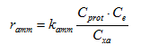
The ammonification of proteins is considered to be proportional to the concentration of proteins, to the concentration of hydrolytic enzymes and inversely proportional to the acidogenic biomass concentration. Proteins are regarded as particulate matter with surface area limitations.
Consumption of monomers by acidogens
Equation 6.48
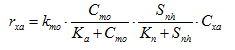
The consumption rate of monomers is assumed to be proportional to monomers and to ammonia nitrogen saturation functions and to the concentration of acidogenic biomass.
Consumption of VFAs by methanogens
Equation 6.49
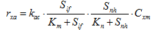
The consumption rate of volatile fatty acids is considered to be proportional to the volatile fatty acids and ammonia nitrogen saturation functions and to the concentration of methanogenic biomass.
Decay of acidogens
Equation 6.50
![]()
The rate of decay of acidogens is assumed to be proportional to their concentration.
Decay of methanogens
Equation 6.51
![]()
The rate of decay of methanogens is assumed to be proportional to their concentration.
Decay of enzymes
Equation 6.52
![]()
The rate of decay of enzymes is assumed to be proportional to their concentration
A schematic diagram of the prefermenter model is shown in Figure 6‑12 (adapted from Munch et al., 1999).
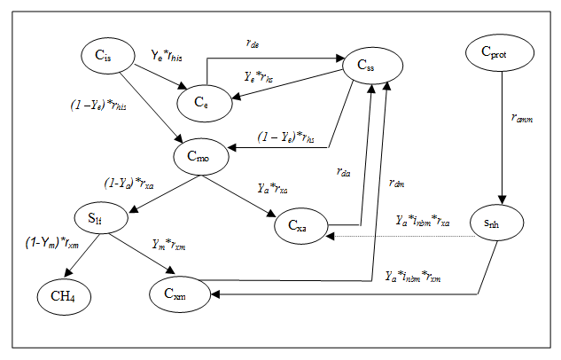
Figure 6‑12 – Schematic Diagram of the prefermenter Model
The Model Matrix for the prefermenter model can be found in Appendix A.
With a large number of models available in the provided literature and used in GPS-X, it can be a challenge to select which model is best for each modelling application. The following simple guide gives a few suggestions and “rules of thumb” for selecting an activated sludge model.
1. The first choice to be made is the GPS-X macro library. If you are only concerned with carbon and nitrogen processes, then you should use the CN (1‑step nitrification) library. If you are interested in modelling phosphorus, then the CNP or Comprehensive libraries should be used. If you are interested in modelling pH, inorganic precipitation and/or side stream processes, use the Comprehensive library. Extra user-defined components can be added to the models by selecting the associated IP (Industrial Pollutant) library – CNIP or CNPIP.
2. It is a good rule of practice to keep the model as simple as possible at the beginning, until you interpret the results and are comfortable with that model's level of complexity. You can then move to more complicated models. If you are unsure of which model to start with we recommend using asm1, or mantis.
3. The choice of model should depend on the amount and type of data that is available to support its use. For example, if you have little information about different substrate types in your system, it is advisable to use models that have fewer substrates.
4. If you are modelling a plant that has recycling of flows back from the solids handling process back to the activated sludge line, the Mantis2 model is best suited for handling this situation. The Comprehensive (Mantis2) library contains a full set of state variables that cover both activated sludge and anaerobic digestion processes.
The choice of model should reflect the need to simulate certain processes. For example, if you are interested in exploring P-removal or alkalinity control, you will need to use models that contain processes that are relevant to those components. Table 6‑2 summarizes the processes in each model, and may be useful in choosing a model. You can consult the model descriptions earlier in this chapter or the Model matrices found in Appendix A to see the details of the processes contained in each model.
Table 6‑2 – Model Processes in GPS-X
*not part of the published model, but added in GPS-X.
The model associated with the deep shaft object is an adaptation of the mantis suspended-growth model. It takes into account the specific hydraulics and hydrostatic pressure found in a deep shaft reactor.
The deep shaft header tank is modelled with two complete-mix reactors (by default), and is under atmospheric pressure. The downcomer and the riser shafts are modelled with twenty complete-mix reactors (by default).
The two membrane bioreactor objects in GPS-X (plug-flow and completely-mixed) are a combination of a suspended-growth activated sludge model, and a simple suspended solids separation filter. They are available in all libraries, and with all biological models. The two MBR objects are shown in Figure 6‑13, with the connection points illustrated.
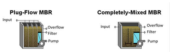
Figure 6‑13 - GPS-X Membrane Bioreactor Objects
The structure of the MBR model combines a conventional activated sludge tank model (plug-flow or CSTR) with an in-tank solids separation filter, as shown in Figure 6‑14. In the case of the plug-flow MBR, the filter is placed in the final tank (an optional internal recycle is shown for illustrative purposes). Permeate flow is drawn through the filter at a rate determined by the filter model.
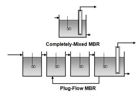
Figure 6‑14 - Membrane Bioreactor Model Structures
The MBR models in GPS-X allow for three modes of operation. The mode of operation can be toggled in the Input Parameters > Model Options menu. The three modes can be set up using the Model Option settings summarized in Table 6‑3.
Table 6‑3 - Settings of MBR Operating Modes
|
Operation Mode |
Backwash and TMP calculations |
Volume Calculations |
|
Simple |
Do not calculate backwash or TMP |
Fixed Volume |
|
Intermediate |
Calculate backwash and TMP |
Fixed Volume |
|
Advanced |
Calculate backwash and TMP |
Variable Volume |
Simple Mode assumes that the filter is properly operated to maintain flux, and does not consider the effects of trans-membrane pressure (TMP), cake formation, fouling, backwashing, and membrane resistance. The Intermediate model mode calculates the TMP, cake formation, fouling, backwashing, and membrane resistance based on the specified backwash rate and cleaning frequency, but the required permeate flux is calculated based on the influent flow and waste flow to ensure that the liquid volume in the last tank remains constant. The Advanced model mode is similar to the Intermediate model mode, however the liquid volume in the tank is variable and can increase or decrease based on the calculated permeate flux. The user can control the liquid level using a feedback controller that manipulates the trans-membrane pressure. Table 6‑4 summarizes the differences between Simple Mode, Intermediate, and Advanced Mode.
Table 6‑4 – MBR Model Modes
|
Operating Parameter |
Operating Mode |
||
|
Simple |
Intermediate |
Advanced |
|
|
Flow Balance and Reactor Volume |
Model assumes flow in equals flow out, and there is no change in reactor volume. All incoming flow is assumed to exit via the filter and waste flow stream |
Required membrane flux is determined based on influent flow and waste flow to ensure the liquid volume in the reactor is constant |
Membrane flux is determined from filter model. Reactor volume increases and decreases depending on the difference between flow in and flow out. A controller is provided to manage the tank level |
|
Filter Operation |
Filter operation is ignored |
Users must specify TMP, backwash/relaxation cycles, and cross-flow aeration |
same as intermediate |
|
Cross-Flow Air |
Filter-cake solids removal from cross‑flow aeration is ignored, but oxygen transfer from the cross‑flow air to the bulk liquid is calculated and included in the biological activity |
Both solids removal and oxygen transfer are considered for cross-flow aeration |
same as intermediate |
|
Solids Capture |
The solids capture rate determines what fraction of the mixed liquor solids remain in the reactor. These solids remain suspended in the bulk liquid. |
The solids capture rate determines what fraction of the mixed solids remains in the reactor. These solids make up the filter cake, and can be returned to the bulk liquid through backwashing or cross‑flow aeration. |
same as intermediate |
|
Biological Activity |
There is no difference in the biological model when using simple, intermediate, or advanced modes. |
||
All physical and operational parameters relating to the specification and operation of the activated sludge reactors are identical to the CSTR and plug-flow tank objects (with one exception – mechanical aeration is not available). The specification of the membrane filter physical characteristics is done in the Input Parameters > Physical – Membrane menu, as shown in Figure 6‑15. All parameters except solids capture rate are ignored (and greyed-out on these menus) when the model is set to Simple Mode.
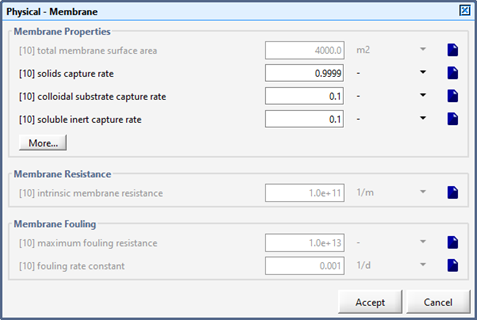
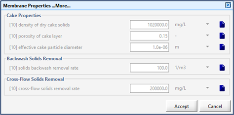
Figure 6‑15 – Physical – Membrane Forms
The GPS-X MBR model calculates the removal of solids due to the
membrane using a mass balance and the solids capture rate (actually
a fraction) specified in the
Input Parameters > Physical – Membrane form.
The default solids capture rate has been selected to provide
a permeate TSS concentration of 1 mg/L or less for typical MBR MLSS
concentrations (i.e. 8,000 to 12,000 mg/L). A separate mass
balance is applied to each particulate component in the biological
model.
In the simple mode, the permeate flow (and flux) is calculated using a volumetric balance and the specified influent and pumped flows. In advanced mode, the permeate flux through the membrane is modelled using a resistance-in-series model (Choi et al., 2000) as shown below:
Equation 6.53
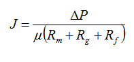
where:
J = permeate flux (m/s)
∆P = trans-membrane pressure (kPa)
μ = viscosity of water (Pa’s)
Rm = intrinsic membrane resistance (m-1)
Rc = cake layer resistance (m-1)
Rf = fouling resistance (m-1)
The trans-membrane pressure, ∆P, is specified in the Input Parameters > Operational ‑Membrane Form, as described in the section below. The viscosity of water is calculated using the following equation (Günder, 2001):
Equation 6.54
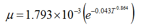
where:
T = temperature (°C)
The intrinsic membrane resistance, Rm, is
provided in the
Input Parameters > Physical – Membrane
form. The default value used is based on data
provided by Chang et al. (1999). In advanced mode,
GPS-X tracks the formation of a cake layer on the surface of the
membrane that resists the liquid flux across the membrane.
The cake layer is assumed to be homogeneous and its thickness is
calculated as shown below in Equation 6.55 (Choi
et al., 2000).
Equation 6.55
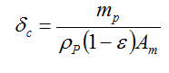
where:
δc = cake layer thickness (m)
mp = dry mass of cake layer (kg)
pP = density of a cake layer particle (kg/m3)
ε = porosity of cake layer (dimensionless)
Am = total membrane surface area (m2)
The dry mass of the cake layer (see Equation 6.54) is calculated using the following dynamic mass balance on the cake layer:
Equation 6.56
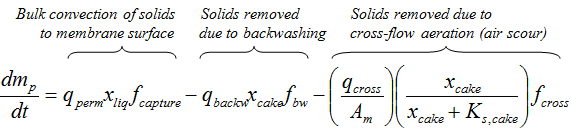
where:
qperm = permeate flow rate (m3/d)
xliq = concentration of solids in bulk liquid phase within the MBR (kg/m3)
fcapture = solids capture rate or fraction (dimensionless)
qbackw = backwash flow rate (m3/d)
xcake = mass of solids in cake layer (kg)
fbw = backwash solids removal rate (1/m3)
qcross = crossflow or air scour flow rate (m3/d)
Am = total membrane surface area (m2)
fcross = cross-flow solids removal rate (kg/m)
Ks,cake = half-saturation coefficient for cross-flow air (kg)
The cake layer mass balance considers the bulk convection of solids to the surface of the membrane, the solids removed due to backwashing, and the solids removed due to cross-flow aeration. Equation 6.55 ignores the diffusion away from the cake layer into the bulk liquid as this term is assumed to be small compared to the other terms in the mass balance. The half-saturation coefficient for cross-flow air and the switching function based on the mass of cake solids is used to smoothly stop the solids removal as the cake layer disappears.
The default density
of a cake layer particle (see Equation 6.54) is equal
to the density of dry biofilm already used in the GPS-X fixed-film
reactors. The default porosity of the cake layer (see
Equation 6.54) is given in the
Input Parameters > Physical – Membrane > More…
form and is estimated using information given in Chang et
al. (1999). The membrane surface area
(see Equation 6.54) is
site-specific and should be selected to achieve a flux within the
range normally recommended by the manufacturer (e.g. a typical
range for hollow fiber membranes is 17 to 25 L/m2/h; see
Wallis-Lage et al., 2005).
The backwash solids removal rate (see Equation 6.55) is specified in the Input Parameters > Physical – Membrane > More … form. It is multiplied in Equation 6.55 by the backwash flow and the cake solids mass (term 2 in Equation 6.55) to give the mass of solids removed from the filter cake per unit time. The default backwash solids removal rate was calibrated using data from Garcia and Kanj (2002). The default backwash flow (see Equation 6.55) is entered in the Input Parameters > Operational – Membrane form and is based on data provided by Garcia and Kanj (2002).
The cross-flow solids removal rate (see Equation 6.55) is the mass of solids removed from the filter cake, per unit of cross flow air, per unit surface area of the filter. The default value is entered in the Input Parameters > Operational – Membrane > More … form and is calibrated based on data in Garcia and Kanj (2002). The cross-flow airflow (see Equation 6.55) is entered in the Input Parameters > Operational – Membrane form. The default value gives airflow per surface area of 0.37 m3/m2/h (see Wallis Lage et al., 2005) for the default membrane surface area. The cross‑flow airflow should be changed to reflect changes in the membrane surface area.
The cake layer resistance, Rc, is calculated by combining Equation 6.54 and the Kozeny-Carman equation for flow through porous passages as follows:
Equation 6.57
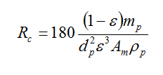
where:
dp = effective cake particle diameter (m)
The default effective cake particle diameter is given in the Input Parameters > Physical – Membrane > More…form, and is estimated using information given in Shin et al. (2002).
The fouling resistance is calculated as follows (adapted from Choi et al., 2000):
Equation 6.58
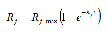
where:
Rf,max = maximum fouling resistance (m-1)
kf = fouling rate constant (d-1)
t = time since last recovery clean (d)
The maximum fouling resistance and fouling rate constant can be found in the Input Parameters > Physical – Membrane > form. They are selected based on data in Merlo et al. (2000). The model assumes that the fouling material is completely removed during a recovery clean so that the time for fouling starts after each recovery clean.
The membrane operational parameters can be set in the Input Parameters > Operational – Membrane form, shown in Figure 6‑16.
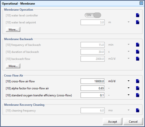
Figure 6‑16 – Membrane Operational Parameters Menu
The trans-membrane pressure from Equation 6.1 is set in this menu, along with the MBR backwashing options (including the frequency, duration and flow rate of the backwash). Alternatively, the level controller can be used, which sets the backwash length to the amount of time required to refill the tank. If the level controller is on and the tank is already full, no backwashing will take place.
A helpful warning alarm can be set in the Membrane Backwash …More… menu. The “warn if tank is overflowing or empty” alarm will print information to the Command Window if the filter flow causes the final tank to overflow or become empty.
A membrane flux controller can be activated to maintain the trans-membrane pressure at the membrane flux setpoint using a built-in controller with the rate of pressure increase being the controller gain.
The cross-flow air used to clean the membranes is assumed to be delivered using a coarse-bubble aeration system. The alpha factor for cross-flow air is based on total suspended solids concentrations of between 8,000 mg/L and 10,000 mg/L in the MBR. The standard oxygen transfer efficiency (cross-flow) is based on a coarse bubble aeration system at submergence of 4.3 m (14 ft.).
The cleaning frequency sets how often physical/chemical cleaning is used to reset the membrane fouling resistance to zero.
Several membrane-specific output variables are available to be plotted. The Membrane Filter Variables menu is accessed from the overflow connection point (not the filter connection point), and is shown in Figure 6‑17.
The MBR Cake Variables menu (shown in Figure 6‑18) provides output variables for total cake mass and cake thickness.
The following points are useful to keep in mind when setting up an MBR simulation:
· When modelling a recycle activated sludge (RAS) stream, the user can simply use the internal recycle feature (located in Operational – Tank > Internal Flow Distribution) and set the internal recycle from the final (membrane) tank to the desired tank.
· Use Simple Mode initially to establish the required operating conditions, such as MLSS, SRT, waste flow, etc.; and in cases where details on the maintenance of the permeate flux are not required. If you are only interested in the biological treatment aspects of the system, use Simple Mode. If you need to also simulate the physical aspects of the filter operation (i.e. different backwash cycles, TMP management, etc.), then Advanced Mode is required.
· When using Advanced Mode, pay close attention to the volume in the reactor(s), as it is easy to either drain or overfill the reactor that contains the membrane filter.
· If you wish to have a membrane “relaxation” period (rather than a backwash period), set the duration and frequency as normal, but set the backwash flow rate to zero. This will cause the permeate flow to cease for the appropriate period of time, but there will be no backwash flow into the tank. This can be done in both the Intermediate and Advanced modes.
· There is no steady-state solution for the model in Advanced Mode. The discontinuous backwashing and cleaning cycles render the model without a true steady equilibrium state (similar to why the SBR object does not have a steady-state solution). When using Advanced Mode, you may wish to run a long dynamic simulation (~100 days) to allow time for the system to reach a cyclic or periodic equilibrium. Due to the fact that there is no backwashing or cleaning in Simple Mode, the steady-state solver can be used.
A summary of the default values of the GPS-X MBR model parameters are shown below in Table 6‑5:
Table 6‑5 – GPS-X MBR Model – Default Parameter Values
|
Model Parameter |
Unit |
Default Value |
Comment/Reference |
|
Solids capture rate |
- |
0.9999 |
Default value was selected to provide a permeate TSS concentration of 1 mg/L or less for typical MBR MLSS concentrations |
|
Density of dry cake solids |
kg/m3 |
1,020 |
Hydromantis (2003) |
|
Porosity of cake layer |
- |
0.15 |
Chang et al. (1999) |
|
Solids backwash removal rate |
1/m3 |
100 |
Calibrated using data in Garcia and Kanj (2002) |
|
Cross-flow solids removal rate |
kg/m |
200,000 |
Calibrated using data in Garcia and Kanj (2002) |
|
Intrinsic membrane resistance |
1/m |
1.0e+11 |
Chang et al. (1999) |
|
Maximum fouling resistance |
- |
1.0e+12 |
Calibrated using data in Merlo et al. (2000) |
|
Fouling rate constant |
1/d |
0.005 |
Calibrated using data in Merlo et al. (2000) |
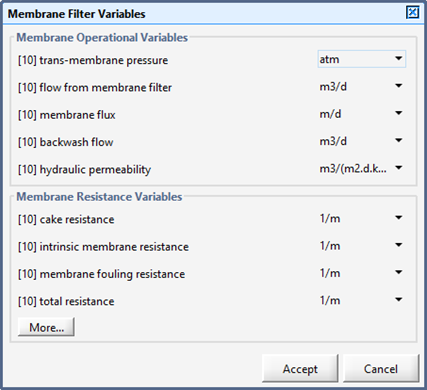
Figure 6‑17 - Membrane Output Variables Menu
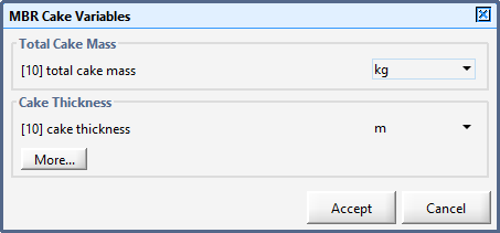
Figure 6‑18 - MBR Cake Variables Menu
The anaerobic MBR model in GPS-X combines the completely-mixed MBR (in simple mode) with the gas transfer and headspace model of the anaerobic digester object. The result is a completely mixed membrane bioreactor with a closed headspace and gas production. Unlike the completely-mixed MBR, there is no modelling of the cake formation on the membrane surface, backwashing of solids, or trans-membrane pressure calculations.
The model assumes that the reactor is completely mixed with no aeration, and that filtrate flow from the MBR is equal to the influent flow minus the pumped flow. It is assumed that the filter is not limiting to the flow (i.e. that whatever flow is calculated can pass through the filter unimpeded). The solids captured by the filter are retained in the completely mixed bulk liquid.
The anaerobic MBR is only available in the Selenium and Sulphur (Mantis2) and the Carbon Footprint (Mantis3) libraries. The anaerobic biological and chemical reactions are identical to those used in the anaerobic digester and UASB models.
The physical menu of the anaerobic MBR object is used to specify the dimensions of the liquid tank and the headspace. In addition, the headspace total gas pressure, gas-liquid transfer constant, and membrane solids capture are specified here as well, as shown in Figure 6‑19 below.
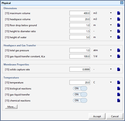
Figure 6‑19 – Anaerobic MBR Physical Parameters Menu
In the Operational input parameters menu, the only operational parameter to be considered is the pump flow rate from the pumped connection on the lower right-hand corner of the object. A PID control loop is available to be configured as well.
The remainder of the menus are similar to those shown in other completely mixed biological reactors.
The output variables available for the anaerobic MBR object are a combination of those from the conventional CSTR and the anaerobic digester. The filtrate and pump connection points show flows, concentrations and operating cost variables for the liquid streams. The gas connection (at the top of the object) shows the gas flow and composition.
The models associated with the sequencing batch reactor (SBR) object are combinations of suspended-growth and sedimentation models. The various aerated and mixed phases use a suspended-growth model, assuming a completely mixed hydraulic configuration, while the settling and decanting phases use a reactive sedimentation model. The models are combined together to form the whole unit process model.
There are three different SBR objects in GPS-X: the simple sequencing batch reactor (SBR) object, the Advanced SBR object, and the Manual SBR object. All three objects have the same functionality, appearance and choice of biological models. They differ in the manner in which the user specifies the operation of the SBR unit.
The simple and advanced SBR objects require the specification of the timing and flow rates to define the phases. The manual SBR object requires that the entire operational cycle be defined by the user, either by having the liquid flows, air flows, and mixing on interactive controllers, or as file inputs. The manual object is suited to operator training, while the simple and advanced objects are typical for an SBR application.
When using multiple, parallel SBRs, it may be desirable to stagger the cycle times of the units. For example, if two parallel SBRs are in use, each with a 6‑hour cycle time, it may be desired to shift one of the SBRs by 3 hours. If both have 3 hours of detention time, then a continuous influent could be switched between the two unit processes. To specify a timeshift for an SBR model using either the simple or advanced objects, the user enters the desired timeshift for the timeshift for simple and advanced cycles parameter. The timeshift parameter cannot be set to a value greater than the cycle time.
The parameters used to specify the operational cycle (in the regular SBR object, not advanced or manual) are found in the Parameters > Operational – Cycle Settings menu. These parameters include the duration of one complete cycle and associated seven separate phases, which have predefined functions. The parameters are shown in Figure 6‑20.
The seven fixed phases for each cycle are described below Figure 6‑20.
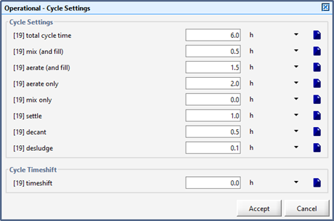
Figure 6‑20 - Regular SBR - Operation Cycle Parameters
1. Mix (and fill): The unit is modelled as a CSTR without aeration (i.e. air flow, power or KLa set to 0.0). This phase is usually the starting phase, used while the tank has just started filling with liquid. This phase represents the first of four mixing phases.
2. Aerate (and fill): The unit is modelled as a CSTR with aeration. This represents the second mixing phase, and is used while the tank is filling after the aeration has been turned on.
3. Mix only: The unit is modelled as a CSTR without aeration. This represents the third mixing phase usually occurring sometime after the tank has finished filling. It is typically used as a denitrifying phase.
4. Aerate:The unit is modelled as a CSTR with aeration. This is the last mixing phase generally used to re-aerate the sludge so that it will settle properly.
5. Settle:The unit is modelled as a settler, with or without biological reactions, depending on the model selected. The mixing is turned off to allow the content of the tank to become quiescent and to promote settling.
6. Decant: The unit is modelled as a settler. During this phase, the user-specified decant flow is activated.
7. Desludge:The unit is modelled as a settler. This phase occurs at the end of the cycle, and the user-specified wastage flow is activated.
With the normal SBR object, the seven phases making up this cycle are fixed in sequence (the order is shown in the form). The total length of all seven phases must not exceed the cycle time specified. If the total length of all seven phases adds up to less than the cycle time, the tank will be idle until the end of the cycle time. If it adds up to a value greater than the cycle time, the remaining time and/or phases beyond the cycle time will be ignored. A phase can be disabled by setting its length to zero.
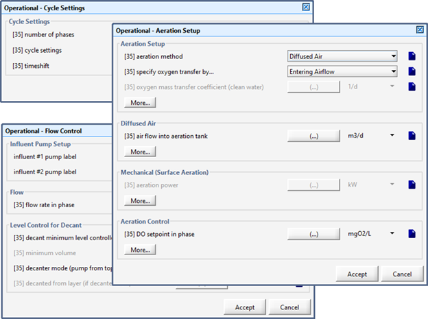
Figure 6‑21 - Advanced SBR Operational Parameter
The decant flow rate (pumped flow parameter) and waste flow rate (underflow rate parameter) are entered in the Parameters > Operational - Flow Control form.
The influent flow to the SBR is taken from the upstream object (e.g. influent object) if the influent #1 pump label parameter is left blank in the Flow Control form. The user must then make sure that the influent flow is synchronized with the SBR cycle (i.e. entering the SBR during the appropriate phase). Alternatively, in the Flow Control form, you can enter a stream label for the influent #1 pump label parameter, a flow rate for the first influent flow parameter, and the SBR influent flow will be automatically taken from that stream during the appropriate phase within the cycle (automatic synchronization). The stream label must be associated with a pumped flow stream (`qcon' variable), for example an influent icon or pumped flow from a tank. The influent #2 pump label parameter is ignored in this cycle type.
The SBR operational cycle parameters for the Advanced SBR model are shown in Figure 6‑21. The advanced SBR cycle is more general than the simple SBR model, allowing the user to define up to ten or more different phases. For each phase defined, the corresponding duration, mixing (either on or off), aeration (oxygen mass transfer coefficient), decant flow rate, and wastage flow rate can be specified. The order of the user-defined phases is fixed according to their order presented in the forms.
The influent flow to the SBR is taken from the upstream object (e.g. influent object) if the influent #1 pump label and influent #2 pump labelparameters are left blank in the Flow Control form. The user must then make sure that the influent flow is synchronized with the SBR cycle (i.e. entering the SBR during the appropriate phase). Alternatively, you can enter stream labels for the influent #1 pump label and influent #2 pump label parameters in the Flow Control form, flow rates for the influent #1 flow in phase and influent #2 in phase parameters in the form (Advanced section), and the SBR influent flow will be synchronized automatically.
The stream labels must be associated with pumped flow streams (`qcon...' variables), for example an influent icon or pumped flow from a tank. Most applications will only use one influent, but second influent was provided for cases were methanol is added, for example.
If the manual SBR object is used, the user must set up all the important parameters such as air flow rate, mixing, decant flow rate, and waste flow rate on interactive controllers to change them as the simulation proceeds.
Alternatively, the parameters can be set up as file inputs or controlled from custom code in the .usr file.
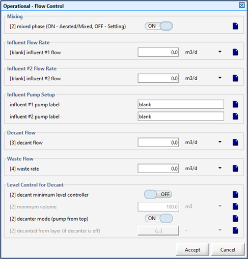
Figure 6‑22 - Manual Cycle Operational Parameters
In the manual SBR model, there are no cycle settings as in the simple and advanced models. The timing of mixing, aeration and pumping all must be controlled directly.
The decant flow rate (pumped flow parameter) and waste flow rate (underflow rate parameter) can be entered in the Parameters > Operational - Flow Control form.
The influent flow to the SBR is taken from the upstream object (e.g. influent object) if the influent #1 pump label parameter is left blank in the Flow Control form. The user must then make sure that the influent flow is synchronized with the SBR cycle (i.e. entering the SBR during the appropriate phase). Alternatively, in the Flow Control form, you can enter a stream label for the influent #1 pump label parameter, a flow rate for the first influent flow parameter, and the SBR influent flow will be automatically taken from that stream during the appropriate phase within the cycle (automatic synchronization). The stream label must be associated with a pumped flow stream (`qcon' variable), for example an influent icon or pumped flow from a tank. The influent #2 pump label parameter is ignored in this cycle type.
The pond object contains only the empiric model, which simulates the transformation, dilution and mixing of state variables in a pond. Unlike the activated sludge models, the empiric model is empirical in nature. It does not use fundamental mechanistic dynamic processes to determine the rate of change of the states (such as those found in the Model Matrices in Appendix A), but simulates behavior that has been observed in existing ponds, bench‑scale studies and pilot-scale studies.
The empiric model simulates three different kinds of ponds: anaerobic, facultative, and aerated. The pond models are discussed in detail below.
Note that Pond/Lagoon object is only available in the GPS-X legacy libraries (cnlib, cniplib, cnplib, cnpiplib)
In the anaerobic pond model, the BOD and TSS removal is simulated using a simple regression model derived from anaerobic pond behavior in North America (Beier, 1987).
The following equations describe the amount of BOD and TSS removal:
Equation 6.59
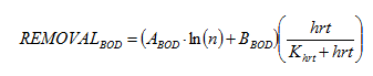
Equation 6.60
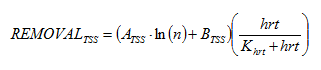
where:
ATSS, ABOD, BTSS, BBOD, Khrt = calibration parameters
n = number of ponds in series
As the empirical equations above only deal with GPS-X composite variables (BOD and TSS), a methodology is required to transfer this information back to the state variables. The following list outlines the relationships for the state variables in CNLIB.
A fraction is calculated for each particulate state variable (xbh, xba, xs, xi, xu, xsto for CNLIB) that is equal to that variable's concentration over incoming xcod.
A new TSS value (x) is calculated from the above empirical REMOVAL equation.
New VSS (vss) and particulate COD (xcod) concentrations are calculated as:
vss = ivt
* x
xcod = icv * vss
A new BOD value is calculated from the above empirical REMOVAL equation, and then compared to the BOD value calculated as the sum of the fractions from step 1 multiplied by the new xcod multiplied by fbod.
If the BOD calculated from the fractions is less than the BOD calculated from the empirical equation, excess soluble BOD (the difference between bod and xbod) is assigned to ss.
If the BOD calculated in step 3 from the fractions is greater than the BOD calculated from the empirical equation, the excess particulate BOD (xbodu) is assumed to be converted to xu. Soluble substrate (and soluble BOD) is then assumed to be zero.
Inert and non-reacting variables are mapped through the pond object (si, salk, and snn).
The effluent oxygen concentration (so) and nitrate concentration (sno) are assumed to be zero in the anaerobic pond environment.
Particulate biodegradable organic nitrogen (xnd) is assumed to be converted to snh as per the conversion of xs.
Soluble biodegradable organic nitrogen (snd) is assumed to be converted to ammonia (snh) as per the conversion of ss.
The loss of heterotrophic (xbh) and autotrophic (xba) biomass results in the production of ammonia (snh).
The approach for facultative ponds is similar to that for anaerobic ponds, but uses a different model for BOD reduction, and a slightly different approach for determining state variable concentrations. The empirical BOD removal model used for facultative ponds is from Thirumurthi (1974):
Equation 6.61
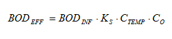
where:
BODEFF = effluent BOD (g/m3)
BODINF = influent BOD (g/m3)
KS = first order BOD removal rate coefficient (1/d) at 20°C
CTEMP = correction factor for temperature
CO = correction factor for organic loading
and
Equation 6.62
![]()
Equation 6.63
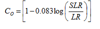
where:
TEMP = temperature, °C
θ = temperature correction constant
SLR = standard loading rate (kg/ha/d)
LR = current loading rate (kgBOD/ha/d)
The methodology for the determination of the state variables xba, xbh, xs, xu, xi, xsto, si, salk, snn, ss, snd and xnd are identical to that for anaerobic ponds.
Oxygen is determined by assuming that the DO is saturated in the aerobic zone, and zero in the anaerobic zone. The concentration of so is determined from the following equation:
Equation 6.64
![]()
where:
SOST = saturated oxygen concentration (gO2m3)
AERDEPTH = fraction of depth that is aerobic (unitless)
For the nitrogen composite variables, nitrate is assumed to be converted to nitrogen gas in the anaerobic zone; therefore:
Equation 6.65
![]()
As anaerobic conversion of biomass and biodegradable nitrogen only happens in a fraction of the pond, the increase in ammonia (snh) as shown in the anaerobic model is multiplied by AERDEPTH.
The aerated pond uses the same empirical BOD and TSS reduction models as the facultative pond model. However, the default value for the BOD removal rate coefficient has been changed to reflect aerated conditions (Eckenfelder, 1980).
The methodology for the determination of the state variables xba, xbh, xs, xu, xi, xsto, si, salk, snn, ss, snd and xnd is identical to that for facultative ponds.
Oxygen is assumed to be saturated at the effluent point of the aerated pond. Due to this completely oxic environment, nitrate is assumed to remain unchanged, and is mapped through the pond object.
Ammonia is assumed not to change, due to the assumption that most of the biomass will be settled out of the water column. Therefore, snh is mapped through the pond object.
The parameters found in the Parameters > Physical page of the pond object include pond type and settings for pond size. Number of cells in series describes the degree of plug flow for the pond system. Typically, BOD and TSS removal increases with increasing numbers of cells in series. The temperature values found on the More... page are used in the temperature correction equations in the facultative and aerated pond models.
The parameters found on the Parameters > Empirical Model Constants include those used to calibrate the BOD and TSS removal, and the half-saturation coefficient KHRT that is used to decrease removal efficiency for very short HRTs.
Table 6‑6 summarizes suggested calibration techniques for the empirical pond models found in the empiric model.
Table 6‑6 – Calibration Suggestions
The above methods for determining the values of state variables from the empirical pond models are for CNLIB only. These methods have been extended to the other libraries by making small additions and changes based on the new and/or different state variables. Table 6‑7 describes these differences.
Table 6‑7 - Library-specific Algorithms for Empiric Pond Model
The oxidation ditch object operation as 16 CSTRs in series (a plug flow tank) with a large recycle from the last tank to the first. The recycle can be specified in four different ways from the Operational menu, using the ditch recirculation mode setting, shown in Figure 6‑23.
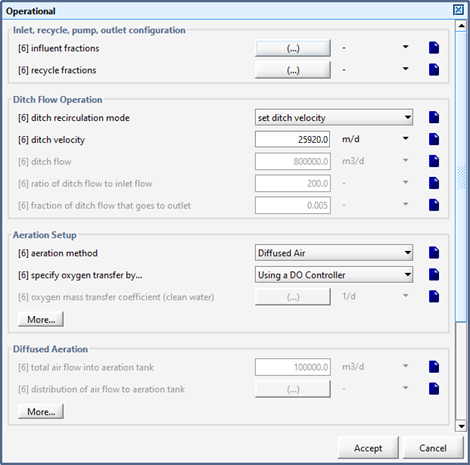
Figure 6‑23 - Oxidation Ditch Recirculation Mode Settings
· Set ditch velocity – specify a constant surface velocity of the ditch flow
· Set constant ditch flowrate – rather than specifying velocity, set the flow
· Set proportional ditch flowrate – make the ditch flow proportional to the incoming flow to the oxidation ditch. Typically, the ditch flow would be 50 to 200 times the incoming flow.
· Set constant outlet fraction – specify the fraction of the ditch flow that exits the ditch each time around.
The oxidation ditch has a series of special two-dimensional output variables that are desiged to be displayed on 2-D greyscale outputs. These variables are found in the 2-D Greyscale Ditch Output output variables menu. These graphs show a plan-view of the oxidation ditch, with tank #1 in the lower right-hand corner, and the effluent point in the upper-right hand corner (the actual influent point depends on the setting in the influent fractions menu). The flow moves clockwise around each ditch.
Five different variables are available for output: Dissolved oxygen (DO), Ammonia, Nitrate, Oxygen uptake rate (OUR) and, Denitrification rate (DNR)
Figure 6‑24 shows an example of the 2-D greyscale DO graph for a typical oxidation ditch.
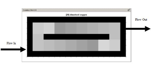
Figure 6‑24 - 2-D Greyscale Oxidation Ditch Output - Dissolved Oxygen
Please Note: Due to the high recycle rate within the object (and subsequent short HRTs for each section of the ditch), the oxidation ditch model often will take longer than normal to converge to steady-state with the steady-state solver. You may find it necessary to increase the iteration termination criteria and/or the damping factor on final approach in the steady-state solver menu to achieve a reasonable solution.
If you are having difficulty with steady-state solutions, you can halt the steady-state solver at a higher iteration termination value, and run a short dynamic simulation to test if the steady-state solver solution is adequate. If the dynamic solution does not diverge appreciably from the steady-state conditions, then the higher iteration termination value is suitable. If you have any questions or problems, please contact us for assistance at support@hydromantis.com
The models associated with the continuous flow sequencing reactor (CFSR) object operates as set of CSTRs in series (a plug flow tank) with a large recycle from the last tank in the series to the first tank. The recirculation flow rate can be specified in 5 different ways from the operational menu, using the recirculation mode setting, shown in Figure 6‑25. The flow moves clockwise around the reactor, in ascending order of CSTR number.
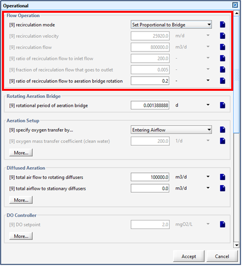
Figure 6‑25 - Continuous Flow Sequencing Reactor Recirculation Settings
· Set recirculation velocity – specify a constant surface velocity of CFSR flow
· Set constant recirculation flowrate – rather thatn specifying velocity, set the flow
· Set proportional recirculation flowrate – make the CFSR flow proportional to the incoming flow to the CFSR.
· Set constant outlet fraction – specify the fraction of the flow that exits the CFSR each time around.
· Set proportional to bridge – set the recirculation rate proportional to the rotational period of the aeration bridge (simulate rotaing aeration brigde does not have to be on for this option to function)
Please Note: Due to the high recycle rate within the object (and subsequent short HRTs for each section of the reactor), the CSR model often will take longer or fail to converge to steady-state with the steady-state solver. You may find it necessary to increase the iteration termination criteria in the steady-state solver menu to achieve a reasonable solution.
If you are having difficulty with steady-state solutions, you can halt the steady-state solver at a higher iteration termination value, and run a short dynamic simulation to test if the steady-state solver solution is adequate. If the dynamic solution does not diverge appreciably from the steady-state conditions, then the higher iteration termination value is suitable. If you have any questions or problems, please contact us for assistance at support@hydromantis.com.
The CFSR consists of a circular tank with an aeration grid suspended from a rotating bridge, though stationary aeration grids can be installed on the floor along the perimeter of the tank. When modelling the rotating aeration bridge, airflow specified in the total airflow to rotating diffusers is moved around the tank from one CSTR cell to the next over the specified rotational period. The rotational period of aeration bridge specifies the period of time required for the rotating diffusers to make one revolution around the tank.
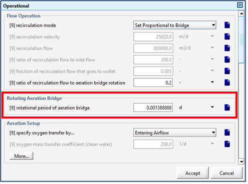
Figure 6‑26 - Continuous Flow Sequencing Reactor Rotating Aeration Bridge Setting
The CFSR object specifies oxygen transfer by using either a DO controller option or entering airflow as the manipulated variable in place of KLa (similar to other DO controllers in GPS‑X). The PID DO controller manipulates KLa and back calculates the required airflow.
The CFSR object contains one additional specify oxygen transfer by... option: The DO On/Off Controller is switches the airflow into the tank on and off depending on the specified DO high and low limits. How quickly action is taken by the controller (after the upper or lower limit is reached) is dependent on the controller’s specified sampling time.
The CFSR object in GPS-X contains three additional Aeration Controllers which can be paired with any of the specify oxygen transfer by... options: timer, nitrate controller and the ammonia controller. These additional controllers can be seen in Figure 6‑27. While the specify oxygen transfer by... controller options control only the DO concentration, the aeration controllers manage more complex aeration strategies in the tank. During aerated phases of each of the aeration controllers, the selected specify oxygen transfer by... option manipulates the airflow according to the following strategies:
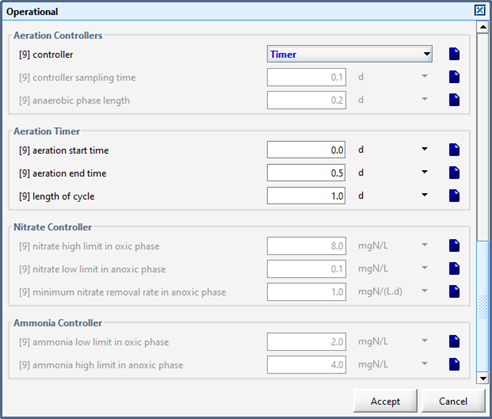
Figure 6‑27 - Continuously Flow Sequencing Reactor Additional Aeration Controllers
· Timer – The timer controller creates a fixed cycle of timed aerated and un-aeratred phases. The timer controller is configured by specifying the aeration start time, the aeration end time, and the length of the entire cycle, where the remaining time in the cycle is un-aerated.
· Ammonia controller – The ammonia controller controls airflow by turning on the air when the ammonia reaches the ammonia high limit in anoxic phase, and turns off the air when the ammonia reaches the ammonia low limit in oxic phase.
· Nitrate controller – The nitrate controller consists of three phases: Oxic, anoxic, and anaerobic:
o Oxic – During the oxic phase, the aeration system in the CFSR is on. Aeration in the tank continues until the nitrate high limit in oxic phase, nitrate concentration, is reached. Upon reaching the specified upper concentration limit, the controller switches to the anoxic phase.
o Anoxic – During the anoxic phase, the aeration system in the CFSR is off. The anoxic phase continues until the nitrate low limit in anoxic phase is reached. Upon reaching the specified low concentration, the controller switches to the anaerobic phase. If the average nitrate removal rate across the CSR drops below the minimum nitrate removal rate in anoxic phase before reaching the low nitrate concentration, the controller will end the anoxic phase and return directly to the oxic phase without executing the anaerobic phase.
o Anaerobic – The anaerobic phase is a time phase of specified duration, commencing at the completion of the anoxic phase. During the anaerobic phase, the aeration system in the CFSR is off. Once the length of time specified in the anaerobic phase length has passed, the controller will return to the oxic phase.
The high purity oxygen (HPO) activated sludge object works the same way as a plug-flow tank object, except that the aeration system uses a HPO gas feed instead of regular air. In addition, the entire plug flow system is capped, and each reactor has a headspace. The headspaces are connected, to allow downstream flow. The flow of gas downstream is determined from the gas input and venting flows, and equalizes the pressure in all the reactor headspaces. Figure 6‑28 shows the physical configuration of the HPO system
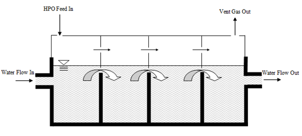
Figure 6‑28 - Schematic of High Purity Oxygen (HPO) System
The flow of gas and flow of water are modelled separately. The exchange of O2 gas, N2 gas and CO2 gas at the air/water interface is determined using Henry’s Law, corrected for temperature and headspace pressure.
The regular biological models have been supplemented in the HPO object with stoichiometry to calculate CO2 gas generation. As the gas travels downstream, O2 is transferred into the liquid and consumed by the biological activity. N2 and CO2 are generated, and equilibrated with the gas concentrations in each headspace. Consequently, the composition of the gas (fraction of the gas that is O2, N2 and CO2) can be displayed for each reactor in the plug-flow system. Output variables for the gas composition can be found in the HPO System Variables output variables menu.
As the HPO system is capped, and CO2 gas is contained in the headspace at concentrations often much higher than atmospheric values, HPO systems may have atypical pH. The GPS-X HPO object contains a pH calculator that determines the pH in the liquid for each reactor. For details on the pH model, refer to the pH discussion in the “Tools” chapter (the model in the Toolbox is the same one used here). It is important to properly specify the anion and cation concentrations in the tank to achieve a calibrated pH calculation.
The pH that is determined for each reactor can be set to inhibit biological growth, using the pH inhibition settings in the Physicalparameters more… button. The pH inhibition is set to OFF by default.
The growth of biomass is multiplied by a pH inhibition factor, taken from Grady and Lim (1980), which is bounded between zero and one. This creates a linear decline between pH = 7.2 and pH ≈ 6.1.
Equation 6.66
![]()
The open basin HPO unit process models the gas-liquid transfer processes for a pure oxygen fed activated sludge process. The open basin systems are considered to provide good oxygen transfer efficiency while allowing better exchange of CO2. The better exchange of CO2 prevents excessive drop in pH. The open basin HPO model has the following features:
1. A gas-liquid transfer model based on feed gas and outlet gas composition
2. Temperature estimation model based on energy balance
3. High temperature and kinetic parameter relationship
Typical outputs from the energy balance model and the oxygen transfer model are shown in Figure 6‑29 and Figure 6‑30.
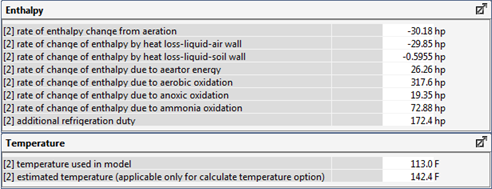
Figure 6‑29 - Typical Outputs from the Energy Balance Model for Temperature Estimation
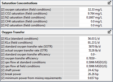
Figure 6‑30 - Typical Outputs for the Oxygen Transfer Rate
The gas transfer to the bulk liquid phase of a biological reactor is modelled using a dynamic mass balance written for each dissolved gas (Hydromantis, 2011). For example, a dissolved oxygen mass balance around a completely stirred tank reactor (CSTR) is shown below.
Equation 6.67
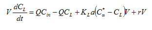
where:
V = reactor volume (m3)
CL = concentration of dissolved oxygen (DO) in the reactor (mg/L)
Q = influent flow rate (m3/d)
Cin = concentration of DO entering reactor (mg/L)
KLa = oxygen mass transfer coefficient at field conditions (1/day)
C*∞ = DO saturation concentration at field conditions (mg/L)
r = rate of use of DO by biomass (g/day), the respiration rate
The volume, flows, and reaction rates are known from specifications or other modelling equations, leaving two terms that must be calculated in order to solve the dissolved oxygen mass balance over time for the DO concentration in the reactor, CL:
1. DO saturation concentration at field conditions, C*∞, and
2. Oxygen mass transfer coefficient at field conditions, KLa
The DO saturation concentration at field conditions is calculated as follows:
Equation 6.68
![]()
where:
τ = temperature correction factor (unitless)
β = correction factor for sales, particulates, and surface-active substances (unitless)
Ω = pressure correction factor (unitless)
C*∞20 = DO saturation concentration at 20°C and 1 atm (mg/L)
The correction factors are used to adjust the DO saturation concentration to account for the temperature of the liquid, the pressure at the submergence level of the diffusers, and the salts, precipitates, and surface-active substances found in the wastewater.
The temperature correction factor is calculated as follows:
Equation 6.69

where:
C*st = surface DO saturation concentration at temperature of t and 1 atm air pressure (mg/L)
C*s20 = surface DO saturation concentration at 20°C and 1 atm pressure (mg/L)
The surface DO saturation concentration at liquid temperature t and an air pressure of 1 atm is obtained using a look-up table in GPS-X that is based on temperature. The look-up table data were taken from Appendix C of the USEPA Design Manual – Fine Pore Aeration Systems (USEPA, 1989). When the temperature falls between two data points in the table, GPS-X uses linear interpolation to determine the C*st value. The value of C*s20 is 9.09 mg/L.
The correction factor for salts, particulates, and surface-active substances, β, is a parameter that must be measured or estimated for the wastewater of interest. In GPS-X, a default value of 0.95 is used.
The pressure correction factor is calculated as follows:
Equation 6.70
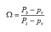
where:
Pb = barometric pressure at elevation and air temperature (kPa)
Ps = standard barometric pressure (101.325 kPa)
pv = vapour pressure of water at liquid temperature (kPa)
The barometric pressure at elevation and air temperature is calculated using the following formula taken from Appendix B-2 of Metcalf and Eddy (2003):
Equation 6.71
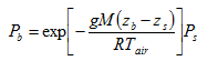
where:
g = acceleration due to gravity (9.81 m/s2)
M = molecular weight of air (28.964 kg/kg-mole)
R = universal gas constant (8314 N•m/kg-mole•K)
Tair = air temperature (K)
zi = elevation at position “i” (m)
The vapour pressure of water at the liquid temperature is determined using the Antoine equation (Felder and Rousseau, 1986):
Equation 6.72
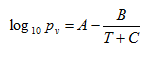
where:
A, B, C = Antoine coefficients
T = wastewater temperature (°C)
The depth correction factor for oxygen saturation is calculated as follows:
Equation 6.73
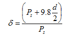
where:
d = depth of the tank
The DO saturation concentration at 20°C and 1 atm is calculated as follows:
Equation 6.74
![]()
The η for each gas is estimated using the following expression:
Equation 6.75
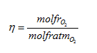
where:
molfro2 = average mole fraction of oxygen in bubble (-)
molfratmo2 = mole fraction of oxygen in air (-)
The average mole fraction of oxygen in the bubble is estimated as below:
Equation 6.76
![]()
where:
molfrffeedO2 = mole fraction of oxygen in feed gas (-)
molfrfoutO2 = mole fraction of oxygen in out gas (-)
wffeed = weight factor for averaging (-, default values is 1.0)
The final expression for the DO saturation concentration at field conditions is as follows:
Equation 6.77
![]()
GPS-X provides four different ways to specify the user inputs to estimate gas-liquid transfer in the open basin HPO system.
1. Direct specification of the clean water at KLa at 20°C
2. Specifying the gas flow rate at standard condition of 1 atm pressure and 20°C temperature
3. Specify the wire point input of the oxygenator
4. Use a DO controller
In each of the above, the user has the option of specifying SOTE. The default value for SOTE for high purity oxygen is considered to be 90%.
Estimate KLa at field conditions
The KLa at field conditions is calculated using Equation 6.11:
Equation 6.78
![]()
where:
KLaT = mass transfer coefficient at temperature T in °C (1/day)
KLa20 = mass transfer coefficient at 20°C
θ = temperature correction factor (default value GPS‑X is 1.024)
α = wastewater correction factor for KLa20
F =diffuser fouling factor (default value in GPS-X is 1.0)
T = wastewater temperature (°C)
Estimate Oxygen Transfer Rate (OTR) at Field Conditions in g/d
Equation 6.79
![]()
Estimate Standard Oxygen Transfer Rate (SOTR) in g/d
Equation 6.80
![]()
Airflow at Standard Conditions in m3/d
The gas flow is calculated usingEquation 6.81:
Equation 6.81
where:
molfrO2 = mole fraction of O2 in user-defined air (mole/mole)
MWO2 = molecular weight of O2 (32 g/mole)
Puser = density of user-defined air (g/m3)
MWuser = average molecular weight of user-defined air (g/mole)
Estimate Airflow rate at Field Conditions
The airflow at standard conditions is converted to field conditions using the ideal gas law:
Equation 6.82
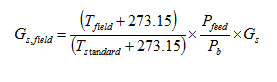
where:
Tstandard = air temperature at standard conditions (°C)
Tfield = air temperature at field conditions (°C)
Estimate the SAE
The SAE is estimated based on the correlation provided by Praxair. The expression is valid for SOTE in the range of 86% to 100%. If the user specified SOTE is less than 80%, then SAE is bounded at 7.11 kg/kWh.
Equation 6.83
![]()
where:
SAE = Specific aerator energy (wire), kgO2/kW-hr
SOTE = Standard oxygen transfer rate (%)
The mechanical power requirement is estimated using the following expression:
Equation 6.84
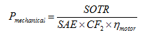
where:
Pmechanical = mechanical power (kW)
SAE = mechanical aerator oxygen transfer rate (kg O2/kW·h)
CF2 = conversion factor (24,000)
ηmotor = motor efficiency
The gas flow rate is entered at a given standard condition of 1 atm and 20°C.
Standard Oxygen Transfer Rate (SOTE) in g/d
The SOTR is calculated using Equation 6.85:
Equation 6.85
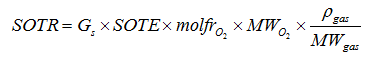
where:
molfrO2 = mole fraction of O2 in feed gas (mole O2/mole gas)
MWO2 = molecular weight of O2 (32 g/mole O2)
Pgas = density of feed gas (g/m3)
MWgas = average molecular weight of gas (g/mole gas)
Estimate OTR
The OTR is calculated using Equation 6.86:
Equation 6.86
Estimate KLa at Standard Condition
Equation 6.87
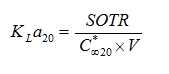
Estimate KLa at Field Condition
Equation 6.88
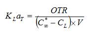
Airflow at Standard Conditions in m3/d
The gas flow is calculated usingthe following expression:
Equation 6.89
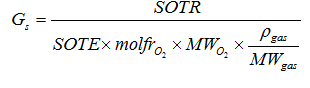
where:
molfro2 = mole fraction of O2 in feed gas (mole O2/mole gas)
MWO2 = molecular weight of O2 (32 g/mole O2)
Pgas = density of feed gas (g/m3)
MWgas = average molecular weight of gas (g/mole gas)
Estimate Airflow Rate at Field Conditions
The airflow at standard conditions is converted to field conditions using the ideal gas law:
Equation 6.90
where:
Tstandard = air temperature at standard conditions
Tfield = air temperature at field conditions (°C)
Estimate the SAE
The SAE is estimated based on the correlation provided by Praxair. The expression is valid for SOTE in the range of 86% to 100%. If the user specified SOTE is less than 80% then the SAE is bounded at 7.11 kg/kWh.
Equation 6.91
![]()
where:
SAE = Specific aerator energy (wire), kgO2/kW-hr
SOTE = Standard oxygen transfer rate (%)
The mechanical power requirement is estimated using the following expression:
Equation 6.92
where:
Pmechanical = mechanical power (kW)
SAE = mechanical aerator oxygen transfer rate (kg O2/kW·h)
CF2 = conversion factor (24,000)
ηmotor = motor efficiency
Estimate the SAE
The SAE is estimated based on the correlation provided by Praxair. The expression is valid for SOTE in the range of 86% to 100%. If the user specified SOTE is less than 80% then the SAE is bounded at 7.11 kg/kWh.
Equation 6.93
![]()
where:
SAE = Specific aerator energy (wire), kgO2/kW-hr
SOTE = Standard oxygen transfer rate (%)
Estimate the SOTR
The mechanical power requirement is estimated using the following expression:
Equation 6.94
![]()
where:
Pmechanical = mechanical power (kW)
SAE = mechanical aerator oxygen transfer rate (kg O2/kW h)
CF2 = conversion factor
ηmotor = motor efficiency
Estimate OTR
The OTR is calculated using Equation 6.95:
Equation 6.95
Estimate KLa at Standard Condition
Equation 6.96
Estimate KLa at Field Condition
Equation 6.97
Airflow at Standard Conditions in m3d
The gas flow is calculated using Equation 6.98:
Equation 6.98
where:
molfro2 = mole fraction of O2 in feed gas (mole O2/mole gas)
MWO2 = molecular weight of O2 (32 g/mole O2)
Pgas = density of feed gas (g/m3)
MWgas = average molecular weight of gas (g/mole gas)
Estimate Airflow rate at Field Conditions
The airflow at standard condition is converted to field conditions using the ideal gas law:
Equation 6.99
where:
Tstandard = air temperature at standard conditions
Tfield = air temperature at field conditions (°C)
Estimate KLa at field condition
The KLa at field conditions is calculated by the controller
Estimate KLa at standard condition
Equation 6.100
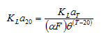
where:
KLaT = mass transfer coefficient at temperature T in °C (1/day)
KLa20 = mass transfer coefficient at 20°C
q (T-20) = temperature correction factor (default value in GPS-X is 1.024)
aF = wastewater correction factor for KLa20
F = fouling factor (default value in GPS-X is 1.0)
T = wastewater temperature
Estimate Oxygen Transfer Rate (OTR) at Field Conditions in g/d
Equation 6.101
![]()
Estimate Standard Oxygen Transfer Rate (SOTR) in g/d
Equation 6.102
![]()
Airflow at Standard Conditions in m3d
The gas flow is calculated using Equation 6.103:
Equation 6.103
where:
molfro2 = mole fraction of O2 in feed gas (mole O2/mole gas)
MWO2 = molecular weight of O2 (32 g/mole O2)
Pgas = density of feed gas (g/m3)
MWgas = average molecular weight of gas (g/mole gas)
The airflow at standard condition is converted to field conditions using the ideal gas law:
Equation 6.104
where:
Tstandard = air temperature at standard conditions
Tfield = air temperature at field conditions (°C)
Estimate the SAE
The SAE is estimated based on the correlation provided by Praxair. The expression is valid for SOTE in the range of 86% to 100%. If the user specified SOTE is less than 80% then the SAE is bounded at 7.11 kg/kWh.
Equation 6.105
![]()
where:
SAE = Specific aerator energy (wire), kgO2/kW-hr
SOTE = Standard oxygen transfer rate (%)
The mechanical power requirement is estimated using the following expression:
Equation 6.106
![]()
where:
Pmechanical = mechanical power (kW)
SAE = mechanical aerator oxygen transfer rate (kg O2/kW h)
CF2 = conversion factor
ηmotor = motor efficiency
The open basin HPO considers the gas-liquid transfer of O2, CO2, N2, H2 and CH4 in Mantis2 model. In Mnatis3 model, gas liquid transfer of N2O is also modeled. The partial pressure of each gas at the surface of the tank is estimated by assuming a virtual gas headspace having a volume equivalent to the volume of the gas holdup in the tank. The virtual head space thus represents the volume in the tank occupied by the bubbles.
The volume of the virtual headspace is estimated by using the following expression:
Equation 6.107
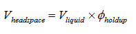
where:
Vheadspace = volume of headspace (m3)
Vliquid = volume of liquid in tank (m3)
Φholdup = gas holdup in tank (-)
The partial pressure of each gas in the headspace is then integrated using the following derivative equation:
Equation 6.108
where:
gi,o = partial pressure of i gas, atm
ptotal = total pressure of the gas in headspace (atm)
rg,i = gas transfer rate for i gas, mole/m3/d
Vliquid = volume of liquid, m3
fmolarvolume = molar volume of gas at standard condition
gi,in = partial pressure of feed gas, atm
Qgas, in = feed gas flow rate, m3/d
Qvent = outlet gas flow rate, m3/d
In general, the relationship between the growth kinetics and the temperature may be expressed using an asymmetrical bell shaped curve. The crest of the curve represents the maximum growth rate at optimum temperature. The growth rate on either side of the crest decreases according to some appropriate growth rate-temperature relationship.
There are a number of models which may be applied to model the temperature dependent kinetics for biological reactions. Depending on the structure of the model, the model may require estimation of model parameters which may be very different than the traditional temperature coefficient approach used in the wastewater engineering. Generally, the Arrhenius equation is used to model the temperature effect on kinetic parameters in the range of 5oC-35oC. This equation requires one parameter of temperature coefficient. The values of temperature coefficients are well researched. Therefore, using any other model which deviates from this relationship will require recalculating of model parameters. To model such a curve the following three parameter model was used.
1. Estimate the kinetic coefficient at the optimum temperature – The kinetic parameter values in GPS-X are listed at 20°C; therefore, this value is translated to a value at the optimum temperature using the following equations:
Equation 6.109
![]()
Equation 6.110
![]()
where:
kopt = kinetic coefficient at Topt, unit
k20 = kinetic coefficient at 20°C, unit
Topt = optimum temperature at which the value of kinetic coefficients is maximum, °C
θ1 = Arrhenius coefficient for low temperature
θ2 = Arrhenius coefficient for high temperature
2. Estimate the value of kinetic coefficient at a given temperature T by using the following equations:
Equation 6.111
![]()
Equation 6.112
![]()
where:
kT = kinetic coefficient at T, unit
T = actual temperature °C
Based on the above relationships the temperature dependency of the kinetic coefficients can be expressed as shown in Figure 6‑31. For the low temperature range, the default GPS-X temperature coefficient values were used for all the kinetic parameters. For the high temperature range temperature coefficient (θ2), the default values of 1.15 and 1.25 were used for the growth rate of heterotrophic and autotrophic microorganisms respectively.
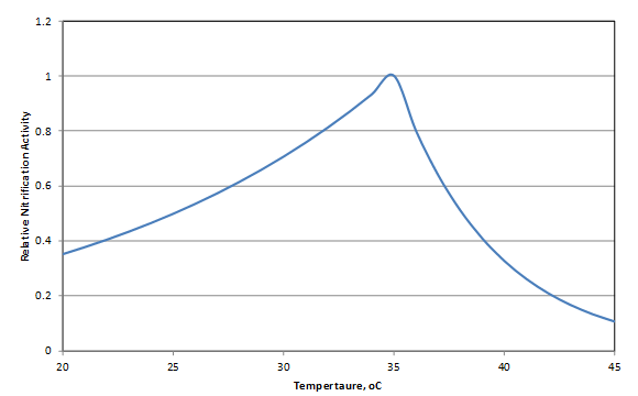
Figure 6‑31 - Variation of Nitrifier Kinetic Parameter Values with Temperature
The current GPS-X model uses a user-defined temperature in the biological unit processes. In using these models, it is assumed that the user has previous knowledge about the expected temperature in different biological reactors. In this project, it was decided to estimate the temperature in the biological units based on the heat balance in the tank considering heat losses and gains.
A simple heat balance model as proposed by van der Graff (1976) and later validated by Gillot and Vanrolleghem (2003) was used to model the temperature change in a biological tank. The model was appropriately modified to account for the heat generation in denitrification and nitrifications reactions. The details of the model are described in following sections.
The equations described in Gillot and Vanrolleghem (2003) were developed for a completely mixed basin under steady state conditions. These equations were appropriately modified to model the temperature under dynamic conditions. The completely mixed hypothesis assumes that the water temperature is uniform over the basin, and equals the outlet temperature. The energy balance over the reactor can be expressed with following equation.
Equation 6.113
![]()
where:
V = volume of the reactor, m3
pw = density of water, kg/m3
cpw = the specific heat of water, J/kg/°C
Qw = the wastewater flow rate, m3/s
Twi = the influent temperature, °C
Two = the water temperature in reactor, °C
ΔH = enthalpy change due to heat transfer, J/s
The ΔH term includes the following terms :
1. Convective and evaporative loss at the surface of the reactor due to aeration. (Hi)
2. Heat loss due to conduction across the reactor wall (Htw)
3. Heat input due to mechanical and blower energy (Hp)
4. Heat input due to biological heat production (Hb)
The calculation method for each heat transfer term is shown in Table 6‑8. The present model neglects the heat transfer due to solar radiation and long wave radiation. The surface convection and evaporation losses are lumped into the convection and evaporative heat transfer due to aeration.
Table 6‑8 – Heat Transfer Terms with Equations for Estimation
|
Heat Transfer Term |
Equation Used for Estimation |
Comment |
|
Hi |
Ui.A.(Ta-Two) |
Convective and evaporative loss during aeration |
|
Htw = Htlaw + Htlsw |
Htlaw =UlaAla(Two-Ta) Htlsw =UlsAls(Two-Ts) |
Heat transfer liquid/air contact wall Heat transfer liquid/soil contact wall |
|
Hp |
Paer |
Power input of surface aerator or blower |
|
Hb = Hbaer+ Hbdn+ Hbaut |
Hbaer = Huaer*rOU Hbdn = Hudn*rDN Hbaut = Hunr*raut |
Heat generation from the aerobic oxidation Heat generation from denitrification Heat generation from nitrification |
The list of parameters used in the temperature estimation model is shown in Table 6‑9.
Table 6‑9 – Parameters for the Temperature Model
|
Parameter |
Description |
Unit |
Value |
|
Ui |
Heat coefficient |
W/m2/C |
Subsurface aeration, Ui = 25 Surface aeration, Ui = 11.4.Paer/V |
|
A |
Surface area of reactor |
m2 |
Variable |
|
V |
Volume of the reactor |
m3 |
Variable |
|
Ta |
Air temperature |
C |
Variable |
|
Two |
Water temperature in reactor |
C |
Variable |
|
Ula |
Heat transfer coefficient for liquid/air wall |
W/m2/C |
1.0 (default) |
|
Ala |
Liquid-air contact wall area |
m2 |
Variable |
|
Uls |
Heat transfer coefficient for liquid/air wall |
W/m2/C |
1.0 (default) |
|
Ts |
Soil temperature |
C |
Variable |
|
Als |
Liquid-soil contact wall area |
m2 |
Variable |
|
Paer |
Total aerator power |
W |
Variable |
|
Huaer |
Unit heat production during aerobic reaction |
J/g O2 consumed |
13985.0 (default) |
|
Hudn |
Unit heat production during denitrification |
J/g NO3-N consumed |
32000.0 (default) |
|
Huaut |
Unit heat production during nitrification |
J/g NH4-N consumed |
25000.0 (default) |
|
rou |
Oxygen uptake rate |
g O2 consumed/s |
Estimated by model |
|
rdn |
denitrification rate |
g NO3-N consumed/s |
Estimated by model |
|
raut |
Ammonia oxidation rate |
g NH3-N oxidized/s |
Estimated by model |
All the heat transfer terms are estimated, and the heat balance equation is solved is solved both for steady state and dynamic conditions. An iterative Newton-Raphson method is used to solve for temperature at steady state.
The powdered activated carbon (PAC) object is a normal CSTR object that has been enhanced with powdered activated carbon addition. The carbon sorbs one or more components using a competitive sorption isoterm. The sorbed components are then coverted to particulate inerts before moving downstream. The version of the PAC model is different in the IP libraries, where 3 user-defined components can be added to the existing sorbable set of state variables, and used as toxic inhibitors to biological activity.
Note the Powdered Activared Carbon object is only available in the GPS-X legacy libraries (cnlib, cniplib, cnplib, cnpiplib)
In the CN and CNP libraries, the only components being sorbed from solution onto the PAC are ss (soluble substrate) and si (soluble inerts). In this two-component system, the sorption rates are:
Equation 6.114
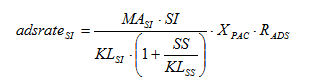
Equation 6.115
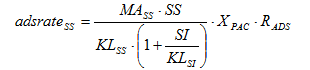
where:
adsrateSI = adsorption rate of SI (gCOD/m3/d)
adsrateSS = adsorption rate of SS (gCOD/m3/d)
MASI = maximum sorption capacity for SI (gCOD/gPAC)
MASS = maximum sorption capacity for SS (gCOD/gPAC)
KLSI = SI sorption half-sat coefficient (gCOD/m3)
KLSS = SS sorption half-sat coefficient (gCOD/m3)
XPAC = PAC concentration in liquid (gPAC/m3)
RADS = adsorption rate (1/d)
The PAC model calculates the amount of “fresh” PAC (PAC that is available to sorb components), and “used” PAC (PAC that has components sorbed onto it, and is not available to sorb more), and the fraction of total PAC that is “fresh” and available to sorb.
The model calculates the concentrations of individual components that are bound to PAC. For PAC-bound soluble substrate, the biomass will grow at an enhanced rate, due to the presence of a concentrated substrate source. This enhancement of growth is controlled by the bioregeneration factor, by which all of the biological growth rates (that grow on ss) are multiplied. The consumption of PAC-bound ss frees up the “used” PAC to become “fresh” PAC again.
In the CNIP and CNPIP libraries, the above-described functionality is enhanced by the addition of user-defined toxic components and their sorption properties. Users can use the IP library versions of the PAC object to investigate the relationship between toxic inhibition and PAC addition to sorb the toxics.
The growth rates for biomass (both heterotrophic and autotrophic) in the Mantis biological model is appended with a switching function for the presence of toxic inhibitors. The user must identify which components are the toxic components, and specify the relative inhibition of each component. The Toxic Inhibition menu contains the parameters used in the inhibition switching function. Figure 6‑32 shows the Toxic Inhibition menu, with sza (IP state variable “soluble component ‘a’”) filled in as Toxic Component #1.
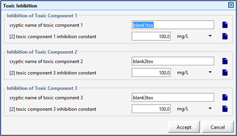
Figure 6‑32 – Toxic Inhibition Menu
Note, the user must specify the cryptic variable name without labels. The user may specify any state variable as a toxic component, including regular states (sno, snh, xnd, etc.) and any of the IP state variables (sza, szb, xza, xzb, etc.).
The toxic component # 1 inhibition constant is a half-saturation coefficient that represents the concentration at which the biological growth rate will be half of its normal value.
The sorption parameters for the toxic components are found in the PAC Addition menu, in the More… button. These components are added to the ss and si sorption isotherms described above, to make a 5-component competitive sorption system. The sorption rates for a five-component system are all on the form.
Equation 6.116
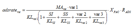
where:
var1, var2, var3 = toxic component concentrations (g/m3)
MAvar = maximum adsorption capacity (g/gPAC)
KLvar = sorption half-saturation coeff (g/m3)
The multi-component competitive sorption model will favour sorption of those components with the lowest sorption half-saturation coefficient.
This chapter describes the aerobic attached-growth models available in GPS-X. These models are associated with the trickling filter, rotating biological contactor (RBC), submerged biological contactor (SBC), simple/advanced biological aerated filter (BAF) and hybrid (IFAS or MBBR) objects. The biofilm model is also used in the anoxic denitrification filter object in the Tertiary Treatment process model group.
The major difference between these models and the suspended-growth models described in Chapter 6 (page 95) is the inclusion of the diffusion process in the biofilm. Although diffusion occurs in suspended-growth systems (substrate and oxygen must diffuse into the activated sludge floc), it is usually neglected since the rate limiting steps are the biological reactions; however, in attached-growth processes, the diffusion and biological reactions must be considered, increasing the complexity of the models.
The trickling filter, RBC, SBC and hybrid processes are similar. They provide biofilm biological treatment, with excess biofilm sloughing separated in a clarifier object. The SBC and BAFs are flooded processes, with mechanical supplemental aeration.
The BAFs differ from the other processes in that it:
· is a combined biological and solids separation process, and
· has a mechanical process for controlling excess biomass growth and captured solids (i.e. backwash)
The advanced BAF model is a combination of an attached-growth model, and a filtration model. The filtration model is described in the One-Dimensional Models section of CHAPTER 8.
The trickling filter model is available in all the libraries, using the same biological reactions found in the suspended-growth models in the appropriate library. The model can predict the extent of carbon and nitrogen removal (by uptake or oxidation) and denitrification, and phosphorus uptake and release. This model incorporates the growth kinetics and transport processes for the corresponding state variables. The profiles of the various components through the biofilm are modelled so that different environments (aerobic, anoxic and anaerobic) can exist within the biofilm.
To reduce the complexity of the model, some assumptions are necessary. The limitations of this model concern the hydraulics of the trickling filter and the biofilm itself. The model assumes that the flow rate and solids loading to the filter can always be processed; that is, clogging and head losses through the filter are not modelled. Also the maximum thickness of the biofilm is not calculated, rather the user specifies it. This assumption was made because there are little or no data available for calibration/verification of the maximum film thickness calculations. It is assumed that there is equal flow distribution over the entire surface area of the trickling filter and the media inside the trickling filter. The effect of the rotation speed of the rotary distributor is neglected.
The dimensions of the trickling filter model are larger than the suspended-growth models since the state variables are now modelled through the film as well as down through the trickling filter. The suspended-growth models only considered the state variables along the reactor (1-dimensional). The additional dimension in the biofilm has some impact on the simulation speed; therefore, more time is required when using this model. Improvements to the speed of this model have been made by integrating the state variables with different frequencies. For example, the particulate components were found to change more slowly than the soluble components since they are diffusing through the biofilm. Therefore, the integration of the soluble components was handled differently from the particulate components (see Figure 7‑3).
The trickling filter is divided into ‘n’ horizontal sections (default is six sections) each representing a cross-section of the trickling filter at a different depth. The transfer of the state variables between each of these horizontal sections through the liquid film is through liquid flow. The biofilm in each of these horizontal sections is modelled as a number of layers (default is one layer for the liquid film on top of five layers for the biofilm). The transfer of soluble state variables between each of these layers is by diffusion only. Particulate variables have a certain physical volume associated with them and can be displaced into the neighbouring layer by growth processes.
Each layer of the biofilm is modelled as a CSTR with the same biological reactions as the suspended-growth biological model (See Appendix A for the mantis model). Attachment and detachment coefficients are used to provide for a means of transfer of particulate components between the biofilm surface and the liquid film. This conceptualization is shown in Figure 7‑1. The concentration of each particulate state variable is converted to volume based on the dry material content of biofilm and the density of biofilm (both user inputs). When the volume of each layer is filled (based on maximum biofilm thickness and number of biofilm layers) the next layer begins to fill. When the film thickness approaches the specified maximum, increasing detachment of biofilm will occur.
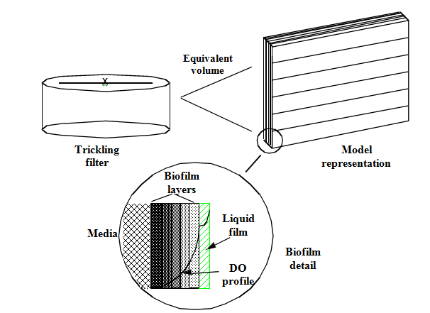
Figure 7‑1 - Conceptual Diagram of the Tricking Filter Model
The mathematical equations used within each layer of the biofilm are provided in the corresponding Model matrix (for example, see Appendix A for the mantis model). The equation used for the diffusion of the state variables from the bulk liquid into the biofilm is provided below. The diffusion through the biofilm is described by Fick's second law and supplemented with biological reactions:
Equation 7.1
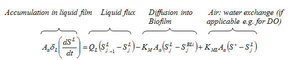
where:
Aa = surface area of biofilm through which transport is occurring (m2)
δL = thickness of attached liquid layer (m)
SjL = substrate conc. in liquid film horizontal section (mg/L)
t = time (days)
S jBLi = substrate concentration at biofilm liquid interface section j (mg/L)
So = saturated liquid-film substrate concentration (mg/L)
QL = volumetric flow rate of attached liquid layer (L/d)
K M = mass transfer coefficient from liquid to biofilm (m/d)
K ML = oxygen transfer coefficient from air to liquid film (m/d)
Equation 7.2
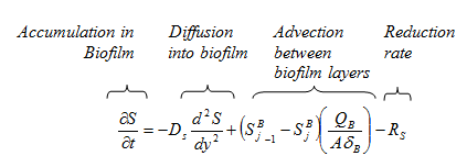
where:
A = surface area of attached microorganisms (m 2)
DS = state variable diffusion coefficient (m2/d)
QB = volumetric flow rate of attached biofilm layer (L/d)
Rs = substrate utilization rate (mg/L/d)
S = state variable concentration in layer (mg/L)
S jB = state variable concentration in attached biofilm layer j (mg/L)
y = thickness of biofilm layer (m)
dL = attached biofilm thickness in layer (m)
This section of the chapter discusses the various model parameters and inputs that the user would encounter when using this model. The examples and discussion below pertain to the mantis model in the CN library.
These menu items are found under the Parameters sub-menu item Physical and contain both real physical dimensions to describe the actual trickling filter being modelled, as well as model dimensions which allow the user to specify how the physical system will be modelled. There are two items under the heading Speed, which allow the user to optimize the simulation speed of this model by changing the frequency of integration for the soluble components.
As seen in Figure 7‑2, the real dimensions of the trickling filter require inputs such as: the filter bed depth, filter bed surface and specific surface of media. Together, these three parameters will provide an estimation of the total biofilm surface area in the model. The liquid retention time in filter refers to the retention time of the liquid flowing past the biofilm, the maximum attached liquid film thicknessrefers to the liquid film which is not moving past the biofilm due to friction (no-slip layer) and the maximum biofilm thickness will be reached only with infinite sloughing. The density of biofilm and dry material content of biofilmare used to convert the concentration of each state variable to a volume measurement.
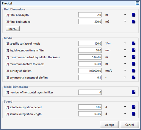
Figure 7‑2 - Physical Dimensions of the Tricking Filter
The model dimensions are fixed, that is, the number of layers in the biofilm is six (one liquid layer and five biofilm layers). Also, the number of horizontal and vertical sections in the model is fixed at six and one respectively.
The next two items in this form, under the heading Speed, concern the integration of the soluble state variables. Since these variables are diffusing through the biofilm, and consequently change rapidly when compared to the particulate state variables, which are changing only due to their growth rates, they tend to dominate the numerical solver. To increase the speed of simulation, the soluble states can be integrated less frequently without loss of accuracy. When the variables are scheduled to be integrated their derivatives are calculated from equations (Equation 7.1) and (Equation 7.2) shown above. Otherwise, the derivatives are set to zero. There are two variables used to specify how frequently the soluble states are integrated and the duration for integration or how long the states are integrated for each period: the soluble integration period and soluble integration length. These concepts are shown in Figure 7‑3 with the results on ammonia shown in Figure 7‑4.
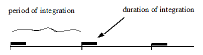
Figure 7‑3 - Integration of Soluble Components
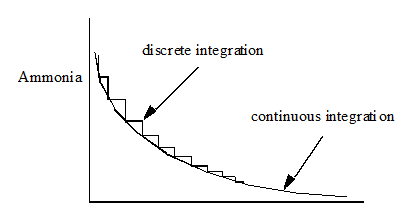
Figure 7‑4 – Integration
The parameters shown in Figure 7‑5 are used for the transport model (diffusion) of the various components through the biofilm. Since there are insufficient data in the literature concerning the diffusion of various components through a biofilm, the values used for the diffusion through water are reduced by a constant fraction, shown as reduction in diffusion in biofilm. The default diffusion coefficients shown for water are used for the diffusion of components from the liquid layer to the first layer (outside) of the biofilm. The detachment rate and attachment rate are used for calculating the sloughing rate and particulate components attachment to the biofilm, respectively.
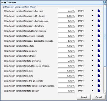
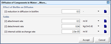
Figure 7‑5 - Mass Transport Parameters
The physical dimensions of the tricking filter show more physical components associated with oxygen. The oxygen mass transfer coefficient is calculated from the physical conditions within the filter (thickness of biofilm and diffusion rate of oxygen) and is affected by temperature and the saturated dissolved oxygen concentration. These values are either input in the general data entry area or specifically set for each object as shown in Figure 7‑6.
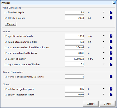
Figure 7‑6 - Physical Dimensions of the Trickling Filter
The parameters shown in these menus refer to the biological reactions that are described in CHAPTER 6 .
In addition to the standard effluent parameters, there are a number of fixed film specific variables that can be displayed. Figure 7‑7 shows the variables available for display for the trickling filter.
This includes the biofilm thickness for each horizontal section from the top to the bottom of the filter.
This provides all the state variables plus the suspended solids composite variable for each horizontal section of the trickling filter (i.e. six profiles for six horizontal sections). The first layer in the profile is the liquid film, followed by the biofilm layers (i.e. liquid and maximum of five biofilm layers).
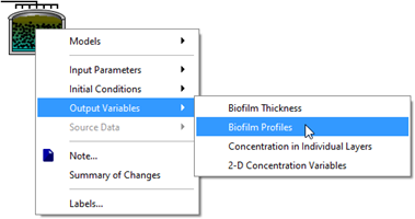
Figure 7‑7 - Tricking Filter Output Variables
This provides the liquid film state variables for each horizontal section of the trickling filter, from top (section 1) to bottom (section 6).
This is used for plotting both the filter horizontal sections and biofilm layers variables using the 3D bar chart or grayscale outputs. Examples are shown in Figure 7‑8. From left to right are the liquid layer and five biofilm layers. In the 3D bar chart, the top of the filter is located in the foreground, and the bottom of the filter in the background. In the greyscale graph, the six horizontal trickling filter horizontal sections are shown from top to bottom (i.e. top layer of the filter is shown at the top of the graph).

Figure 7‑8 - 2D Variables
The rotating biological contractor (RBC) model is available in all the libraries, using the same biological reactions found in the suspended-growth models in the appropriate library. The model can predict the extent of carbon and nitrogen removal (by uptake or oxidation) and denitrification, as well as phosphorus uptake and release. This model incorporates the growth kinetics and transport processes for the corresponding state variables. The profiles of the various components through the biofilm are modelled so that different environments (aerobic, anoxic and anaerobic) can exist within the biofilm.
To reduce the complexity of the model, some assumptions are necessary. The limitations of this model concern the hydraulics of the rotating biological contactor and the biofilm itself. The model assumes that the flow rate and solids loading to the RBC can always be processed; that is, clogging and head loss are not modelled. Also the maximum thickness of the biofilm is not calculated; rather it is specified by the user. This assumption was primarily made because there are little or no data available for calibration/verification of the maximum film thickness calculations. The effect of the rotation speed and direction of the RBC and its impact on media sloughing and aeration requirements is neglected.
Similar to the trickling filter model, the RBC is more complex than the suspended-growth models since the state variables are modelled through the biofilm as well as through various RBC stages.
The rotating biological contactor is divided into ‘n’ stages (default is 1 stage) each representing a baffled RBC system. The transfer of the state variables between each of these stages is through the liquid flow. The biofilm in each stage is modelled as a number of layers (default is one layer as the liquid film on top of five layers as the biofilm). The transfer of soluble state variables between each of these layers is by diffusion only. Particulate variables have a certain physical volume associated with them and can be displaced into the neighbouring layer by growth processes. Each layer of the biofilm is modelled as a CSTR with the same biological reactions as the suspended-growth biological model (See Appendix A for the mantis model). Attachment and detachment coefficients are used to provide for a means of transfer of particulate components between the biofilm surface and the liquid film.
This conceptualization is shown in Figure 7‑9. The concentration of each particulate state variable is converted to volume based on the dry material content of biofilm and its density, both input by the user. When the volume of each biofilm layer is filled (based on maximum biofilm thickness and number of biofilm layers) the next layer begins to fill. When the biofilm thickness starts to approach the specified maximum, increasing detachment of biofilm will occur.
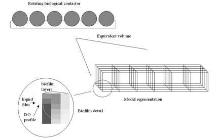
Figure 7‑9 – Conceptual Diagram of the RBC Model
The mathematical equations used within each layer of the biofilm are provided in the corresponding Model matrix (For example, see Appendix A for the mantis model). The equation used for the diffusion of the state variables from the bulk liquid into the biofilm is provided in the trickling filter section.
The mathematical equations used within each layer of the biofilm are provided in the corresponding Model matrix (For example, see Appendix A for the mantis model). The equation used for the diffusion of the state variables from the bulk liquid into the biofilm is provided in the trickling filter section.
These menu items are found under the Parameters sub-menu item Physical and contain both real physical dimensions to describe the actual rotating biological contactor modelled, as well as model dimensions which allow the user to specify how the physical system will be modelled. There are two items under the heading Speed, which allow the user to optimize the simulation speed of this model by changing the frequency of integration for the soluble components. As seen in Figure 7‑10, the real dimensions of the rotating biological contactor require inputs such as the rbc liquid volume, the rbc media volume and the specific surface area of media. Together, these three parameters provide an estimation of the total biofilm surface area in the model. The submerged fraction of the biofilm refers to the percent of the RBC submerged at any given time, the maximum attached liquid film thickness refers to the liquid film which is considered to be associated with the biofilm due to friction (no-slip layer), and the maximum biofilm thickness will be reached only with infinite sloughing. The density of biofilm and dry material content of biofilm are used to convert the concentration of each state variable to a volume measurement. The model dimensions include the number of RBC tanks in series or stages. The model assumes each tank or stage is of equal size. If the stages are of unequal size (different media density and/or parallel feeding), the user should tie individual RBC objects together to simulate the process.
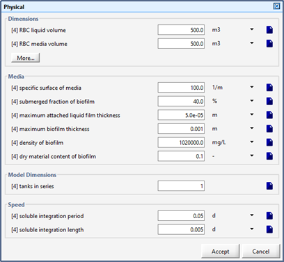
Figure 7‑10 - Physical Dimensions of the RBC
The next two items in this form, under the heading Speed, concern the integration of the soluble components. Since these components are diffusing through the biofilm, and consequently change rapidly when compared to the particulate components, which are changing only due to their growth rates, they tend to dominate the numerical solver. To increase the speed of simulation, it was found that these components can be integrated less frequently without loss of accuracy. When the soluble variables are scheduled to be integrated, their derivatives are calculated from equations (Equation 7.1) and (Equation 7.2). Otherwise, the derivatives are set to zero. There are two variables which are used to specify how frequently the states are integrated: the soluble integration period, and the duration for integration or how long the states are integrated for each period (soluble integration length). These concepts are shown in Figure 7‑3, with the results for ammonia shown in Figure 7‑4.
Figure 7‑11 shows more physical components associated with oxygen solubility. The oxygen mass transfer coefficient is calculated from the physical conditions within the filter (thickness of biofilm and diffusion rate of oxygen) and is affected by temperature and the saturated dissolved oxygen concentration. These values are either input in the general data entry area or specifically set for each object.
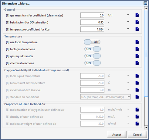
Figure 7‑11 – Physical Dimensions of the RBC (More…)
The parameters shown in Figure 7‑5 are used by the RBC for the transport model (diffusion) of the various components through the biofilm. Since there are insufficient data in the literature concerning the diffusion of various components through a biofilm, the values used for the diffusion through water are reduced by a constant fraction, shown as reduction in diffusion in biofilm. The default diffusion coefficients shown for water are used for the diffusion of components from the liquid layer to the first layer (outside) of the biofilm. The rate of detachment and attachment is used for calculating the sloughing rate and particulate components attachment to the biofilm.
The parameters shown in these menus refer to the biological reactions that are described in CHAPTER 6.
In addition to the standard effluent parameters, there are a number of fixed film specific variables that can be displayed. These are accessed through the object’s Output Variables menu item.
· RBC Variables (see Trickling Filter Variables section in this chapter)
· Liquid Concentrations (see Liquid Film Concentrations section in this chapter)
· 2D Variables (see 2D Variables section in this chapter)
The submerged biological contactor (SBC) model is a modification of the RBC model for units that are air driven or are provided with supplemental aeration. Units with supplemental aeration tend to be more submerged than conventional RBCs (conventional RBCs are generally 40 percent submerged) providing additional contact of the media with the influent, since the unit is not dependent on ambient air for oxygen.
The SBC model discussed herein is available in all the libraries, using the same biological reactions found in the suspended-growth models in the appropriate library. The model can predict the extent of carbon and nitrogen removal (by uptake or oxidation) and denitrification, as well as phosphorus uptake and release (in the carbon-nitrogen-phosphorus library). This model incorporates the growth kinetics and transport processes for the corresponding state variables. The profiles of the various components through the biofilm are modelled so that different environments (aerobic, anoxic and anaerobic) can exist within the biofilm.
To reduce the complexity of the model, some assumptions are necessary. The limitations of this model concern the hydraulics of the submerged biological contactor and the biofilm itself. The model assumes that the flow rate and solids loading to the SBC can always be processed; that is, clogging and head loss is not modelled. The maximum thickness of the biofilm is not calculated; rather it is specified by the user. This assumption was made because there are little or no data available for calibration/verification of the maximum film thickness calculations. It is assumed that there is equal flow distribution over the entire surface area of the SBC and the media inside the SBC. The effect of the rotation speed or direction of the SBC and its impact on media sloughing is neglected. The oxygen diffused into the biofilm when the media is in the air is neglected, since the SBC media is generally submerged more than 80 percent of the time; therefore, the SBC is modelled as completely submerged.
Similar to the trickling filter model and the RBC, the SBC is more complex than the suspended-growth models since the state variables are now modelled through the film and through various SBC stages (or shafts).
The submerged biological contactor is divided into a number of stages (default is 2 stages) each representing a baffled SBC shaft. The transfer of the state variables between each of these stages is through the liquid flow. The biofilm in each stage is modelled as a number of layers (default is one layer as the liquid film on top of five layers as the biofilm). The transfer of soluble state variables between each of these layers is by diffusion. Particulate variables have a certain physical volume associated with them and can be displaced into the neighbouring layer by growth processes. Each layer of the biofilm is modelled as a CSTR with the same biological reactions as the suspended-growth biological model (See Appendix A for the mantis model). Attachment and detachment coefficients are used to provide for a means of transfer of particulate components between the biofilm surface and the liquid film.
For the SBC the process is the same as the RBC (conceptually shown in Figure 7‑9). The concentration of each particulate state variable is converted to volume based on the dry material content of biofilm and its density input by the user. When the volume of each layer is filled (based on maximum biofilm thickness and number of biofilm layers) the next layer begins to fill. When the film thickness starts to approach the specified maximum, increasing detachment of biofilm will occur.
The mathematical equations used within each layer of the biofilm are provided in the corresponding Model matrix (for example, see Appendix A for the mantis model). The equation used for the diffusion of the state variables from the bulk liquid into the biofilm is provided in the trickling filter section.
This section of the chapter discusses the model parameters and inputs that the user will encounter using this model, in particular those different from the other fixed film models. The example and discussion below pertains to the mantis model in the Carbon - Nitrogen (CN) library.
These menu items are found under Parameters > Physical, and contain both real physical dimensions to describe the actual submerged biological contactor being modelled, and model dimensions which allow the user to specify how the physical system will be modelled. there are two items under the heading Speed, which allow the user to optimize the simulation speed of this model by changing the frequency of integration for the soluble components.
As seen in Figure 7‑12, the real dimensions of the submerged biological contactor require inputs such as:
1. tanks in series
2. volume set up method
3. SBC liquid volume in tanks
4. SBC media volume in tanks
5. SBC total volume
6. SBC total media volume
7. volume fractions
8. Specific surface of media (which will provide an estimation of the total biofilm surface area in the model.)
Based on the volume set up method (input 2), the user either specifies the individual volumes per tank (inputs 3 and 4), or the volume fractions based on the total volumes (inputs 5, 6 and 7). The latter two items are used to convert the concentration of each state variable to a volume measurement. Model dimensions include the number of SBC tanks in series or stages.
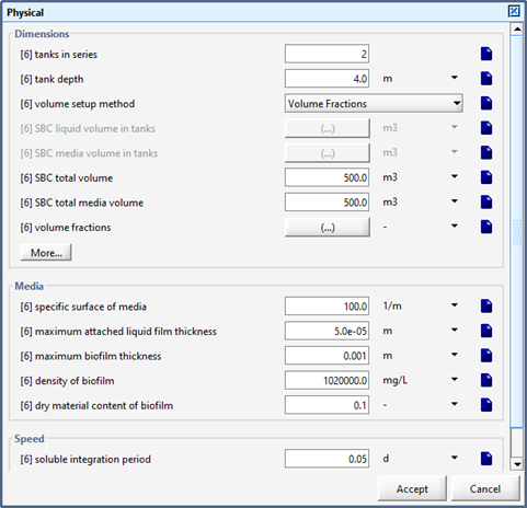
Figure 7‑12 – Physical Dimension of the SBC
Biofilm characteristics include:
1. Maximum attached liquid film thickness, which refers to the liquid film that is considered to be associated with the biofilm due to friction (no-slip layer).
2. Maximum biofilm thickness, which will be reached with infinite sloughing
3. Density of biofilm
4. Dry material content of biofilm
The next two items in this form under the heading Speed, concern the integration of the soluble components. Since these components are diffusing through the biofilm, and consequently change rapidly when compared to the particulate components, which are changing only due to their growth rates, they dominate the numerical solver. To increase the speed of simulation, it was found that these components could be integrated less frequently without loss of accuracy. When the soluble variables are scheduled to be integrated their derivatives are calculated as normal. Otherwise, the derivatives are set to zero. There are two variables which are used to specify how frequently the states are integrated (Soluble integration period) and the duration for integration or how long the states are integrated for each period (Soluble integration length). These concepts are shown in Figure 7‑3, with the results for ammonia shown in Figure 7‑4.
The oxygen mass transfer coefficient is calculated from the physical conditions within the filter (thickness of biofilm and diffusion rate of oxygen) and is affected by temperature and the saturated dissolved oxygen concentration. These values are input in the general data entry area or specifically set for each object as shown in Figure 7‑13.
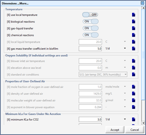
Figure 7‑13 - Physical Dimensions of the SBC (More...)
The operational parameters are similar to the activated sludge model. Like the activated sludge model, the aeration method can be chosen as either “Enter KLa” or “Enter Airflow”. No mechanical method is provided since this method is not appropriate for the SBC.
The parameters shown in Figure 7‑5 are used by the SBC for the transport model (diffusion) of the various components through the biofilm. Since there are insufficient data in the literature concerning the diffusion of various components through a biofilm, the values used for the diffusion through water are reduced by a constant fraction, shown as reduction in diffusion in biofilm. The default diffusion coefficients shown for water are used for the diffusion of components from the liquid layer to the first layer (outside) of the biofilm. The rate of detachment and attachment is used for calculating the sloughing rate and particulate components attachment to the biofilm.
The parameters shown in these menus refer to the biological reactions that are described in CHAPTER 6.
In addition to the standard effluent parameters, there are a number of fixed film specific variables that can be displayed. They are the same as the trickling filter. These are accessed through the following subheadings:
· SBC Variables (see Trickling Filter Variables section in this chapter)
· Liquid Concentrations (see Liquid Film Concentrations section in this chapter)
· 2D Variables (see 2D Variables section in this chapter)
The simple BAF model combines the 1-D biofilm model used in the trickling filter with an aeration model and simple solids-separation model. It is similar in construct to the denitrification filter, with the addition of aeration. The Simple BAF model is designed to be a less-sophisticated, but easier-to-use alternative to the advanced BAF model. The Simple BAF model will solve to steady-state using the GPS-X steady-state solver (whereas the Advanced BAF model cannot, and requires a dynamic simulation to come to equilibrium).
The simple BAF uses a series of horizontal layers (6 by default) to represent plug-flow through media. The filter is fed from the bottom and effluent is taken from the top.
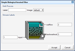
Figure 7‑14 - Simple BAF Model Configuration
Oxygen solubility is calculated separately for each layer, allowing for depth effects to be reflected in oxygen saturation concentration.
Influent flow enters the unit through the lower-left connection point, and exits from the upper right-hand connection point. Solids that are periodically backwashed from the unit are converted to a continuous flow that exits from the lower-right connection point.
The physical parameters menu for the Simple BAF model contains parameters for the description of the unit, including the characteristics of the media. Figure 7‑15 shows the physical parameters menu. The definitions of the various biofilm parameters (e.g. maximum biofilm thickness, etc.) are identical to those described in the section on the Trickling Filter model. The default parameter values for the media characteristics are set for typical BAF media.
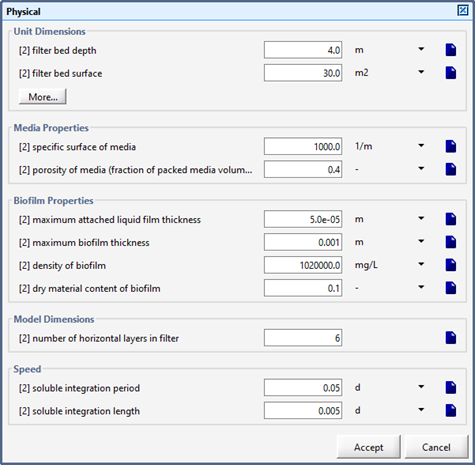
Figure 7‑15 - Simple BAF Model Operational Parameters Menu
The operational parameters menu contains settings for the aeration and backwashing of the filter.
The solids capture fraction is used to determine the mass of solids captured on the filter. These solids are then removed via the
The backwash flow rate and backwash duration per 24-hr period are used (along with the calculated captured solids) to calculate a mass flow of backwashed solids. The backwashed flow is converted from an intermittent event to a continuous flow of equivalent mass solids. This allows for the model to be solved using the steady-state solver.
Details of the aeration setup can be found in the More... button under in the Aeration Setup section. (Figure 7‑16)
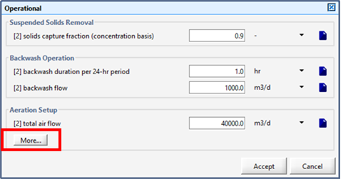
Figure 7‑16 - Simple BAF Model Operational Parameters Menu (More...)
The remaining menus are equivalent to those found in the Trickling Filter Model.
The advanced biological aerated filter (BAF) model is a robust, mechanistically-based model. It uses the same biological reactions found in the suspended-growth models discussed in Chapter 6.
The advanced BAF model consists of four major components: Hydraulics and Filter Operation, Filtration, Biological Reactions, and a Biofilm. They are described in the following sections.
The model needs to be able to describe the complex operation of the bio filter stages each consisting of one or more units in different operating modes.
In the simplest implementation (number of units is 1); the model simulates the behavior of a single BAF unit. This unit can be in filtration, standby, backwash, or flush mode. In filtration, standby and flush mode, the filter is represented hydraulically as a tank consisting of a certain number of horizontal sections (6 in the default case). The actual filtration bed is preceded by a mixed tank without filter material to describe the dilution effects of the volume of water under the filter bed. A similar mixed tank is added to account for the liquid on top of the filter media. In backwash mode the horizontal sections of the filter are combined and converted to one mixed tank. The model assumes that during backwash the filter media is ideally mixed.
The influent loading to the filter determines if the filter is in filtration, standby, backwash, or flush mode. In filtration and flushed modes, flow is entering the filter through the input stream and coming out through the output stream. In standby mode, there is no flow through the filter. In backwash mode, flow is entering the filter through the backwash input stream and coming out through the backwash output stream.
A complex bio filter plant could be represented by the proper number of individual filter units placed on the drawing board to describe the changing conditions in the plant and forecast effluent quality. Due to the level of complexity within one filter unit and the typical number of units in the plant this approach is not feasible even with substantial computing capacity. Since the difference between individual units operating in the same mode is not drastic, a simplified operation mode provides a good approximation of operating and effluent conditions with substantially less overhead.
For this purpose the hydraulics of the filter (which now can be thought of as a series of units) is described in three different ways. A certain fraction of the total number of units is in filtration mode, i.e. layered with influent flowing through them. Another fraction is in standby mode, with light aeration and no influent loading. A third fraction is in backwash mode. The sum of the three fractions adds up to the total number of units. At times any one of these fractions may be completely missing, i.e. the number of units in backwash or standby mode can be zero. In GPS-X, the individual fractions are specified in two ways:
1. As constants – This allows a simple run when the number of units in standby does not change. When a particular backwash criterion is reached, a certain number (user-specified) of units in a filtration mode are backwashed. This mode can be used if an actual operation of a filter plant is recorded and has to be replayed in GPS-X. The number of units can be read in through the GPS-X input file facility, and the original loading conditions recreated.
2. As volume fractions which vary according to a target load on the filter component – This way the ration of the operating filter volume, and the standby volume changes continuously according to changes in influent load. This operation mimics a "constant loading" operational policy, although the loading is completely constant on the filter volume because the limitation created by the individual bio filter unit volumes are ignored.
During the simulation when volume fractions in different operating modes change, the model correctly keeps track of mass balances by recalculating the mass of all model components currently in that element. As an example consider the event of one standby unit coming on-line due to increasing load on the filter. The other elements in the filter, which have been in operation, may contain much higher active biomass than one, which has been on standby for a period of time. When the standby component comes on-line, a volume weighted average biomass concentration is calculated for the new, increased filter volume for all horizontal sections and all biofilm layers, and integration continues using the new conditions.
The modified Iwasaki equation (Horner et al., 1986) was used to calculate the filtration rate, while head loss is calculated according to the Kozeny equation. In the filtration mode, the number of horizontal sections is determined by the plug flow characteristics of the BAF bed (6 by default). This component of the model is used in predicting solids capture, effluent suspended solids and other constituents and backwash quality. In backwash mode, the backwashed fraction of the bed is treated as an ideally mixed tank; biofilm layers are retained.
The filtration element of the model is available without the biological reactions in the current sand-filter model in GPS-X described in One-Dimensional Model section of Chapter 9.
The BAF models use the same biological reactions found in the suspended-growth models in the appropriate library. The mantis model has been successfully used in several biofilm configurations by Hydromantis, and is able to predict ammonia and BOD profiles in the reactor and in the biofilm. For more specific information on biological models, please consult CHAPTER 6.
The existing biofilm model in GPS-X is based on Spengel and Dzombak (1992). This model was adapted to the simple and advanced BAF configurations. The model handles soluble material diffusion, biofilm growth, and particulate attachment and detachment. Details are described in the Trickling Filter Model section of this chapter.
The mathematical equations used within each layer of the biofilm are provided in the corresponding Model matrix (see Appendix A for the mantis model). The equations used for the diffusion of the state variables from the bulk liquid into the biofilm are provided in the Trickling Filter Model section of this chapter. The equations used for the filtration component are provided in the One-Dimensional Model section of CHAPTER 9.
This section discusses the various model parameters and inputs that the user will encounter when using this model.
The physical parameters are found under the Input Parameters sub-menu item Physical. It contains physical dimensions to describe the actual BAF being modelled and model dimensions, which allow the user to specify how the physical system will be modelled. There are three items under the heading Speed, which allow the user to optimize the simulation speed of this model.
As seen in Figure 7‑17, the unit dimensions of the BAF require inputs such as the single filter bed surface area, the total filter bed depth from support, the media fill (empty bed depth) (the difference between the last 2 inputs giving the water height above the media), and the water height below support. The number of units makes the simplified multiple units operation possible.
The next section of this form, media, includes inputs to characterize the media being used in the filter: Specific surface of media together with the filter bed depth and surface area provides an estimation of the total biofilm surface area in the model; Equivalent particle diameter, where multi-media filters can be described; Clean bed porosity (void space); and ultimate bulk biofilm volume, the maximum space the biofilm can take up before completely clogging the filter.
The next two items under the Biofilm heading, density of biofilm and dry material content of biofilm, are used to convert the concentration of each state variable to a volume measurement. The Model Dimensions section includes the number of sections in filter; the model assumes each horizontal section is of equal size.
Figure 7‑17 shows physical components associated with oxygen solubility and model speed. The oxygen mass transfer coefficient is calculated from the physical conditions within the filter (thickness of biofilm and diffusion rate of oxygen) and is affected by the liquid and air temperatures, and the oxygen fraction in air (See CHAPTER 6). These values are input in the general data entry area or specifically set for each object as shown in this screen. The first two items under the heading Speed concern the integration of the soluble components, which is described in the Trickling Filter Model section of this chapter. The third item, calculate DO in liquid, is used to improve the speed of simulation if the BAF installation maintains a relatively high level of DO in the liquid (close to saturation). By setting this parameter to OFF, a constant DO level is maintained in the liquid and integration of the DO state variable is bypassed, thereby speeding up the simulation. The constant DO level can be adjusted in the initial conditions form (Process Data > Initialization > initial concentrations).
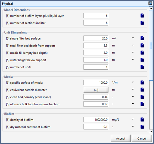
Figure 7‑17 - Advanced BAF Physical Parameters
In the first part of the Operationalmenu item, aeration constants are available similar to all aerated biological units. Specific to the advanced BAF model is the ability to specify a different KLa (or air flow, if the aeration method is set to diffused) for each of the filter operational states (active, standby, flushed, or backwashed). These parameters are shown in Figure 7‑18
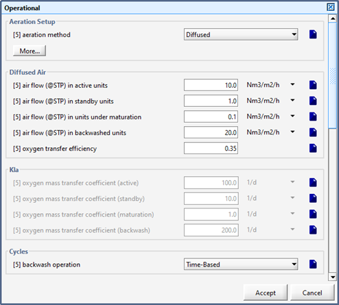
Figure 7‑18 - BAF Operational Parameters
The entry under the Cycles heading, backwash operation, is used to set up the method by which a backwash operation will be initiated when operating the filter(s). The backwashoperation can be time-based, head loss-based, effluent quality based, or manual. The filter can be operated in single unit mode (the whole volume will be in filter, backwash, standby or flushed mode), or multiple unit operation. In multiple unit operation (if the number of units is greater than one), the number of units in filter mode can be specified, and the remaining units are in standby mode. The number of simultaneously backwashed units will be taken out of the filtration mode and replaced with standby units when a backwash operation is initiated if the constant filter loading rate controller is on. The target loading rate on the filter fraction can be specified and thus the volume of filter in filtration mode will vary to maintain the target loading rate.
This form contains further information about the backwash operation. Backwash can be initiated after a certain period (i.e. every 24 hours), or after a maximum allowable head loss is achieved (i.e. 1 m), or when the effluent solids reach a threshold level (i.e. 10 g/m3). This last mode may be useful for optimizing plant performance in the mathematical model. In manual mode, the operation of the BAF has to be done through a Control window (or file input), which needs to be set up with all the operational variables.
Further model parameters are included in the mass transport, stoichiometric, kinetic and filtrationmenu items in the BAF model. These forms are described in the Trickling Filter Model section of this chapter and in the Sand Filtration Models section developed in CHAPTER 9.
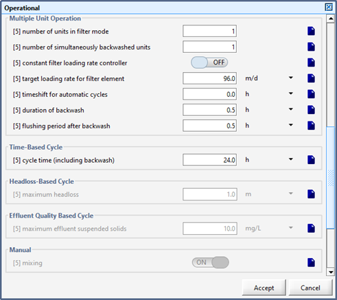
Figure 7‑19 - More Advanced BAF Operational Parameters
Here, hydraulic information can be accessed and displayed for each of the horizontal filter sections (6 by default). It includes dilution rate and headloss-related variables: Reynolds number, friction factor, and headloss in each horizontal filter section for both clean and dirty filter beds.
The solids capture rate during filtration can be displayed for each of the horizontal filter sections. The other variables (O2 partial pressure, pore size, biofilm thickness, deposit concentration, bulk deposit volume) can be displayed on 3D graphs. The x-axis has the six horizontal filter sections, the y-axis has the five biofilm layers and liquid phase, and the z-axis displays the variable value.
The state variables and the solids composite variable can be displayed on 3D graphs. The x-axis has the six horizontal filter sections, the y-axis has the five biofilm layers and liquid phase, and the z-axis displays the variable value.
In this form, the state variables and unattached solids composite variable values in the liquid phase can be selected for display for each of the horizontal filter sections. The values displayed are only valid for the BAF units in filtration mode.
In this form, the state variables can be selected for display for each of the biofilm layers. The values displayed are only valid for the units in backwash mode, and represent the average of all horizontal filter sections. In filtration mode, the filter is treated as a completely mixed tank.
The Hybrid-System model in GPS-X is based on a combination of the standard plug flow tank configuration with suspended growth biomass, and the GPS-X biofilm model representing fixed film growth on the media inserted into the tank. Any type of media will be represented in the model as long as the specific surface area is set correctly. Thus the model is able to represent commercial systems such as MBBR, Ringlace, Captor, Bionet and other types of hybrid systems, whether they contain sludge recycle or not.
The hybrid-system uses the same biological reactions found in the suspended-growth models. For more specific information on biological models, please consult CHAPTER 6.
The existing biofilm model in GPS-X is based on Spengel and Dzombak (1992). This model was adapted to the hybrid-system. The model handles soluble material diffusion, biofilm growth, and particulate attachment and detachment. Details are described in the Trickling Filter Model section of this chapter.
This section of the chapter discusses the various model parameters and inputs that the user will encounter when using this model.
The physical parameters are found under the Parameters sub-menu item Physical. It contains physical dimensions to describe the hybrid-system, and model dimensions which allow the user to specify how the physical system will be modelled.
The hybrid-system requires inputs such as the specific surface of media, the water displaced by media, and the specific density of media.
In the Operational form, aeration constants are available similar to all aerated biological units. Specific to the hybrid-system is the ability to specify two additional recycle streams. These streams are internal recycle with carrier(if internal recycle carries carrier with it) and flow from tank # with carrier (if the carrier can flow from one cell to the next one).
Further model parameters are included in the mass transport, stoichiometric and kinetic menu items in the hybrid-system model. (See Trickling Filter Model section in this chapter)
In addition to the standard initial volume input, the hybrid-system requires the reactor portion filled by media (media or empty bed fill), which can be input in the Initial Volume sub-menu form.
In addition to the standard effluent parameters, there are a number of fixed film specific variables that can be displayed. These are accessed through the object's output variables menu item.
The denitrification filter objects are found in the “Tertiary Treatment” group of objects, rather than in the “Attached Growth” group, as the other biofilm objects.
The denitrification filter model is similar to the trickling filter model in hydraulic structure. There are, however, a few fundamental differences:
1. The filter is assumed to be entirely flooded. There is no empty void space between media, as in the trickling filter model.
2. The trickling filter model is assumed to be downflow, whereas there are two different denitrification filter models: Upflow and Downflow, as shown in Figure 7‑20.
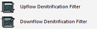
Figure 7‑20 - Upflow and Downflow Denitrification Filter Objects
The denitrification filter model uses the same biological reactions found in the suspended-growth models. For more specific information on biological models, please consult CHAPTER 6.
The existing biofilm model in GPS-X is based on Spengel and Dzombak (1992). This model was adapted for use in the attached-growth objects such as the trickling filter and denitrification filters. The model handles soluble material diffusion, biofilm growth, and particulate attachment and detachment. Details are described in the Trickling Filter Model section of this chapter.
The filtration of solids is modeled as a simple capture of the particulate state variables from the effluent layer of the denitrification filter (bottom layer in the downflow filter and top layer in the upflow filter). Users specify a capture fraction, and all solids captured are removed through the backwash connection stream. Backwashing (and its associated removal of solids) is modeled as a continuous process flow.
This section of the chapter discusses the various model parameters and inputs that the user will encounter when using this model.
The physical parameters are found under the Parameters sub-menu item Physical. It contains physical dimensions to describe the denitrification filter, and model dimensions which allow the user to specify how the physical system will be modelled.
The denitrification filter requires inputs such as the specific surface of media and the porosity of media.
The operational menu contains three parameters that define the removal of solids via backwash. The solids capture fraction defines the fraction of particulate state variables (on a concentration basis) that is removed from the effluent stream. The parameters backwash duration during 24-hr period and backwash flow are used to determine the total amount of flow leaving through the backwash connection point per day. The backwash concentration is calculated as the total amount of captured solids divided by the daily backwash flow rate.
Further model parameters are included in the mass transport, stoichiometric and kinetic menu items in the denitrification filter model. These forms are described in the Trickling Filter Model section of this chapter.
The initialization menu of the denitrification filter object is the same as for the trickling filter object, and contains the initial concentrations of the state variables in each layer of the filter.
In addition to the standard effluent parameters, there are a number of fixed film specific variables that can be displayed. These are accessed through the object's output variables menu item.
The Membrane-Aerated (MABR) object is found in the Attached Growth section of the Unit Process Table.

Figure 7‑21- Hollow Fibre Membrane Aerated Bioreactor object
The MABR object uses a structure similar to the Hybrid object, in that it is a suspended growth reactor with media supporting biofilm growth. Unlike the Hybrid object, the media can only be fixed (as opposed to floating), and the aeration of the biofilm is done from the membrane surface itself (as opposed to via the bulk liquid), effectively aerating the biofilm from the inside out. Regular diffused aeration of the bulk liquid is also available in this object.
Figure 7‑22 shows the structure of the MABR biofilm model. At the left, the media surface area supports the growth of biofilm. The biofilm is modelled as 5 homogeneous layers, followed by an interface with the bulk liquid. Soluble components from the bulk liquid can diffuse into (and out of) the outermost biofilm layer (the one in contact with the liquid). The MABR membrane surface allows for the diffusion of oxygen through the membrane and into the innermost biofilm layer.
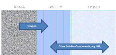
Figure 7‑22 - MABR biofilm structure, showing diffusion of soluble components
As the with the other biofilm models in GPS-X, each of the biofilm layers is modelled as a completely-mixed reactor. All aspects of solids transfer (internal solids exchange, attachment and detachment at the liquid/biofilm interface) are all modelled similar to the hybrid model.
This section of the chapter discusses the various model parameters and inputs that the user will encounter when using this model.
The physical parameters are found under the Parameters sub-menu item Physical. It contains physical dimensions of the MABR unit, and details of the media surface area and biofilm properties.
The total amount of surface area available for growing biofilm is equal to the number of cassettes multiplied by the modules per cassette, cords per module and media length. The surface area per length of media is determined from the media outside diameter and the thickness of the biofilm. Therefore, the surface area per length of media increases with increasing media diameter and biofilm thickness.
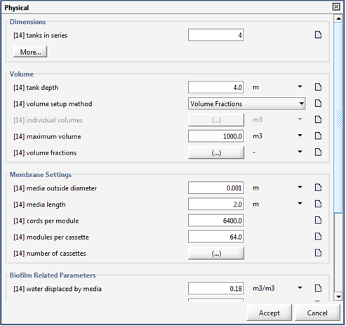
Figure 7‑23 - MABR Physical Parameters Menu
The operational menu contains parameters that define the operation of the membrane aeration, conventional bulk liquid aeration and hydraulic settings (e.g. internal mixed-liquor recycle flow) of the MABR unit.
The first section of the menu, “Inner Biofilm Aeration” contains settings for specifying the mass transfer of oxygen from the membrane to the innermost biofilm layer. There are three options available for specifying oxygen transfer:
1) setting the mass transfer coefficient, kLa, in units of 1/d
2) setting the mass transfer of oxygen directly, in kg/d
3) using the pressure difference equation, which specifies the oxygen transfer through the length of the membrane using inlet and outlet pressure and oxygen fraction
The pressure-difference oxygen transfer model is described by Côté (1989), and is shown below:
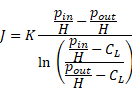
where,
J = oxygen flux, mol/m2-sec
K = mass transfer coefficient, m2/sec
pin = partial pressure of oxygen at inlet, Pa
pout = partial pressure of oxygen at outlet, Pa
H = Henry’s Law constant, Pa-m3/mol
CL = oxygen concentration in liquid, mol/m3
The operational menu for selecting the method for specifying oxygen transfer is shown below.
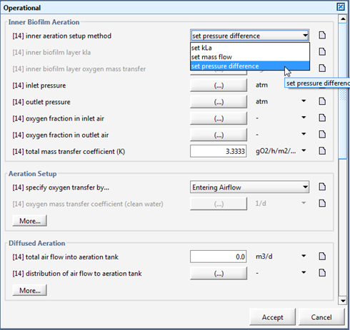
Figure 7‑24 - MABR Operational Menu
Note that the kLa and pressure difference options incorporate the oxygen saturation term into the overall mass transfer, meaning that as the dissolved oxygen in the liquid (or biofilm, in this case) comes closer to saturation, the oxygen transfer decreases. This is not the case for the direct oxygen mass transfer setting. The amount of oxygen (in mass-per-unit-time terms) will be transferred, regardless of oxygen saturation. The user is should note that this can possibly result in the oxygen concentration in the innermost biofilm layers being above saturation.
The default setting for oxygen transfer specification is the pressure difference model.
The mass transport menu of the MABR object contains parameters relevant to the transport of components to, from, and within the layers of the biofilm. The menu is shown below:
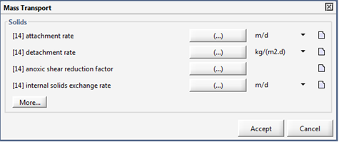
Figure 7‑25 - MABR Operational Menu
These parameters are similar to those used in other biofilm objects:
attachment rate – a rate constant used to determine the mass flow of solids from the bulk liquid to the outermost biofilm layer
detachment rate – a rate constant used to determine the mass flow of solids from the outermost biofilm layer to the bulk liquid
anoxic shear reduction factor – a parameter which reduces the amount of detachment in tanks with no aeration, to simulate the calmer conditions present without diffused aeration
internal solids exchange rate – a parameter used to determine the mass flow of solids between internal layers in the biofilm
For details on how the attachment/detachment and solids exchange rates are calculated, please see the details of the trickling filter model.
The Mass Transport menu also contains further constants for the diffusion of soluble components through the biofilm. These are accessed by clicking on the MORE… button at the bottom of the menu. The menu that pops up contains diffusion constants for each of the soluble components as well as the biofilm reduction factor. The reduction in diffusion constant for each soluble component is treated differently in the MABR model than it is in the other biofilm models in GPS-X. In the other models, there is one biofilm reduction factor that is applied to all the soluble components (default = 0.5). In the MABR model, each soluble component has its own biofilm reduction factor, which can be different from each other. In general, the default values for the different soluble components are 0.2 for organic components, and 0.8 for inorganic components, as per Stewart (2003).
Further model parameters are included in the stoichiometric and kinetic menu items. These forms are described in the Trickling Filter Model section of this chapter.
The initialization menu of the MABR object is the same as for other biofilm objects, and contains the initial concentrations of the state variables in each layer of the biofilm.
In addition to the standard effluent parameters, there are a number of fixed film specific variables that can be displayed. These are accessed through the object's Output Variables menu item.
The MABR Performance Variables menu contains several display unique state variables that illustrate the mass transfer and concentrations of various elements throughout the biofilm. The menu is shown below.
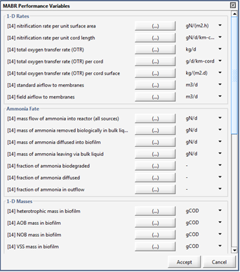
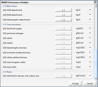
Figure 7‑26 - MABR Performance Variables Menu
The 1-D Rates section contains output variables such as nitrification rate and oxygen transfer rate, calculated in various ways. The Ammonia Fate section summarizes the transformation of ammonia in the reactors of the MABR unit (e.g. how much is removed biologically, how much diffuses into the biofilm, and how much remains in the bulk liquid).
The 1-D Masses and 1-D Mass Flows summarize the distribution and fate of the heterotrophic, ammonia-oxidizing, and nitrite-oxidizing biomass in the bulk liquid and the biofilm. The 2-D Concentrations section contains 2-dimensional array variables of the various soluble and particulate components in the biofilm. These variables are intended to be displayed on a “3D Bar Graph” type, and appear as shown below:
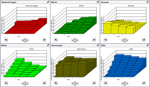
Figure 7‑27 - MABR Performance Variables Menu
In these diagrams, the orientation of the media, bulk liquid and the biofilm layers is shown below:
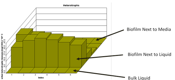
Figure 7‑28 - MABR Performance Variables Menu
This chapter provides a description of the sedimentation and flotation models available in GPS-X.
Sedimentation is one of the most important unit processes in activated sludge treatment plants. The sedimentation unit, whether it is a primary settler, secondary clarifier, or sludge thickener, provides two functions: clarification and thickening. The primary settlers and sludge thickeners are designed and operated to take advantage of the thickening process, while the secondary clarifiers are designed and operated to take advantage of the clarification process.
In GPS-X, the sedimentation models are either zero- (point) or one-dimensional (1d suffix), and either reactive (mantis, asm1...) or nonreactive (simple). The following models are available:
· Zero-dimensional, nonreactive: point
· One-dimensional, nonreactive: simple1d
· One-dimensional, reactive: mantis, asm1, asm2d,asm3, newgeneral
In reactive models, biological reactions are included, and the model names are associated with the corresponding suspended-growth models, described in Chapter 6 (page 95). For example, the mantis sedimentation model uses the mantis suspended-growth model.
In the one-dimensional models, the settler is divided into a number of layers (10 by default) of equal thickness, as depicted in Figure 8‑1.
The following assumptions are made:
1. Incoming solids are distributed instantaneously and uniformly across the entire cross-sectional area of the feed layer.
2. Only vertical flow is considered.
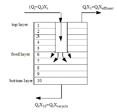
Figure 8‑1 - One-Dimensional Sedimentation Model
The models are based on the solids flux concept: a mass balance is performed around each layer, providing for the simulation of the solids profile throughout the settling column under both steady-state and dynamic conditions.
Table 8‑1 shows the appropriate contribution of each layer of the settler to the mass balance. There are five different groups of layers, depending on their position relative to the feed point. This is shown schematically in Figure 8‑2.
The models are based on traditional solids flux analysis, but the solids flux in a particular layer is limited by what can be handled by the adjacent layer.
The solids flux due to
bulk movement of the liquid is a straightforward calculation based
on the solids concentration times the liquid bulk velocity, which
is up or down depending on its position relative to the feed
layer.
Table 8‑1 – Sedimentation Model: Input-Output Summary
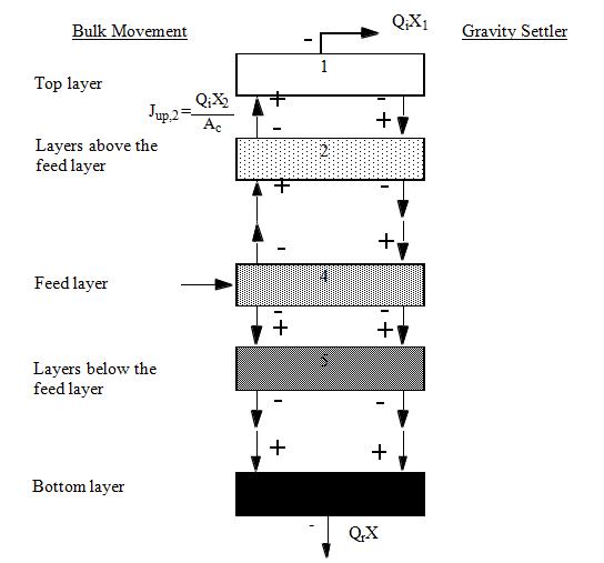
Figure 8‑2 - Solids Balance Around the Settler Layers
The solids flux due to bulk movement of the liquid is a straightforward calculation based on the solids concentration times the liquid bulk velocity, which is up or down depending on its position relative to the feed layer.
The solids flux due to sedimentation is specified by a double exponential settling function, applicable to both hindered sedimentation and flocculant sedimentation conditions. The settling function, described by Takács et al. (1991), is given by:
Equation 8.1
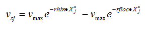
where:
vsj = the settling velocity in layer j (m/d)
vmax = the maximum Vesilind settling velocity (m/d)
rhin = hindered zone settling parameter (m3/gTSS)
rfloc = flocculant zone settling parameter (m3/gTSS)
X jo = Xj – Xmin, where Xmin is the minimum attainable suspended solids concentration, Xj is the suspended solids concentration in layer j
The minimum attainable solids concentration in a layer, Xmin, is calculated as a fraction (non-settleable fraction or fns) of the influent solids concentration to the settler:
Equation 8.2
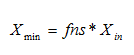
It is subject to a maximum value specified by the user; the maximum non-settleable solidsor Xminmax. The settling velocity is lower bounded to zero, so that if the user specifies parameter values that would result in settling velocities becoming negative, a warning message is printed in the simulation Log window. The settling velocity is also subject to a maximum value specified by the user; the maximum settling velocityor vbnd.
The settling function is shown in Figure 8‑3. The four regions depicted in this figure are explained as follows: I) the settling velocity equals zero, as the solids attain the minimum attainable concentration; II) the settling velocity is dominated by the flocculating nature of the particles; thus the settling velocity is sensitive to the rfloc parameter; III) settling velocity has become independent of solids concentration (particles have reached their maximum size; and IV) settling velocity is affected by hindering and becomes dependent on the rhin parameter (the model reduces to the Vesilind equation).
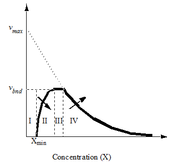
Figure 8‑3 – Settling Velocity vs. Concentration
In the simple1d sedimentation model, the only numerically integrated variable is the suspended solids concentration. This model can be used when biological reactions in the settler can be ignored. The concentrations of particulate state variables in the influent to the settler (heterotrophic organisms, etc.) are stored as fractions of the total suspended solids concentration entering the settler. Once the model completes the numerical integration of the suspended solids in the settler layers (at the end of each numerical integration time step), the concentrations of particulate state variables in the effluent, underflow (RAS), and pumped flow (WAS) are restored using those fractions. The concentrations of soluble state variables are not changed in the simple1d model.
This variable is used to define the sludge blanket height for display purposes. If the concentration in a settler layer is above this threshold value (searching from top to bottom layer), then the sludge blanket is defined as the height of that layer.
This parameter is used to define the height of the sludge blanket in order for the dissolved oxygen in the underflow and pumped streams to be zero.
The soluble state variables in the nonreactive models are subject to a complete mix zone, unlike the particulate components, which move from layer to layer. If the user wishes to subject the soluble components to a number of tanks in series, then they must select a reactive type settler. In this case all of the state variables are transported from cell to cell according to the bulk fluid motion (but only the particulate components will be affected by a settling term). The feed layer then will become an important term in fixing the number of layers in series through which the soluble components will flow.
A feature of the sedimentation models in GPS-X (secondary clarifiers only) is the correlation provided between the settling parameters and Sludge Volume Index (SVI) measurements.
The SVI test characterizes the sedimentation, which occurs in the high solids concentration band of a clarifier. To specify the sedimentation characteristics over the full concentration spectrum, another parameter, the Clarification factor, is needed to specify the settling behavior in the flocculant or low solids concentration regions. This factor is a relative clarification index; a high number (1.0) indicates good clarification and a low number (0.1) indicates poor clarification.
The correlation equations are:
Equation 8.3
![]()
Equation 8.4
![]()
Equation 8.5
![]()
where:
vmax = maximum Veslind settling velocity(m/d)
rhin = hindered zone settling parameter (m3/gTSS)
rfloc = flocculant zone settling parameter (m3/gTSS)
SVI = sludge volume index (mL/g)
clarify = clarification factor
fcorr1 - fcorr9 = SVI correlation coefficients
To use the
correlation, the user must set the parameter use SVI to estimate
settling parametersto ON. The Sludge Volume Index
and Clarification parameters can then be specified and the
settling parameters are calculated automatically by GPS-X. The
correlation coefficients can be accessed in the
Options > General Data > System > Parameters >
Miscellaneous form.
Note: The default values of the correlation factors are for SVI. A correlation with SSVI has not been performed. The default values of the correlation coefficients are based on five sewage treatment plants.
The sedimentation models will account for hydraulic effects caused by an increase in influent flow. Flow conditions are considered normal when the influent flow divided by the surface area is less than the quiescent zone maximum upflow velocity specified by the user. The load to the settler under normal flow conditions enters the settler at the feed layer. However, as the influent flow increases, the load to the settler is distributed to the layers below the feed point. When the upflow velocity in the settler surpasses the complete mix maximum upflow velocity specified by the user, the entire load enters the bottom of the settler.
When the upflow velocity is between the quiescent zone maximum upflow velocity and complete mix maximum upflow velocity, a smooth transition of feed distribution between the low loading case and the high loading case is generated. An average (medium) loading condition is initially calculated where the upflow velocity (vuavg) is the average of the quiescent zone maximum upflow velocity(vumin) and the complete mix maximum upflow velocity(vumax). At this hydraulic loading, the input distribution is equal to the feed layer and all layers below.
Smooth distribution is achieved by two linear interpolations. The first interpolation is between vumin and vuavg. At vumin, the influent fraction to the feed layer is 1.0 (all flow enters the feed layer), while at vuavg the influent fraction to the feed layer is 1.0 divided by the number of layers below the feed layer (including the feed layer itself). Once the influent fraction to the feed layer is calculated, the remaining flow is equally distributed to the layers below.
A similar algorithm will ensure smooth flow distribution above vuavg. The algorithm first calculates the feed fraction to the bottom layer. If vu is higher than vuavg, then the algorithm distributes the rest evenly.
This procedure of flow distribution is modelling the feed distribution to the settler by the influent baffle. The feed distribution is shown in Figure 8‑4.
During higher flows, the momentum of the incoming flow tends to carry the load further past the bottom edge of the influent baffle, effectively changing the feed point in the settler. The flow distribution aspect of the model captures this phenomenon.
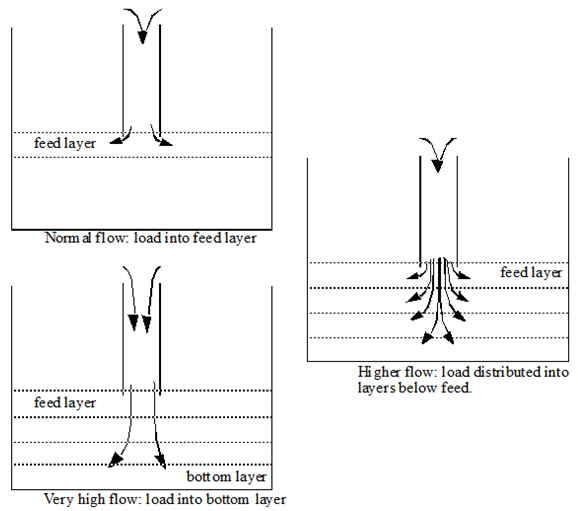
Figure 8‑4 – Load Distribution into Settler
There are four types of settler objects in GPS-X:
1. rectangular primary
2. circular primary
3. rectangular secondary
4. circular secondary
All of the settler objects contain the same settling model. The difference between primary and secondary clarifiers is the default settling parameters and the SVI correlation (SVI correlation is not used in the primary settlers).
The difference between the circular and rectangular configurations is restricted to the specification of the area and/or geometry of the tanks. The rectangular tanks require only a total surface area for input, whereas the circular tanks have several shapes available.
There are 4 different circular settler shapes available in the circular primary and secondary settler objects, as shown in Figure 8‑5. The surface area of each layer is calculated from the clarifier type and dimensions specified by the user. For example, as shown in the figure, a clarifier with a conical shape will have a larger surface area in the upper layer and a smaller surface area in the bottom layer.
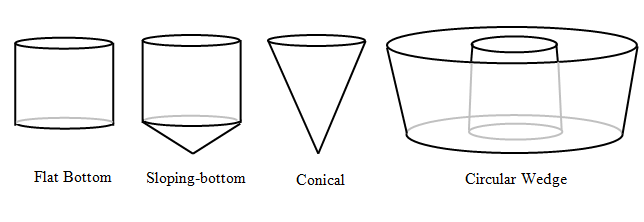
Figure 8‑5 – Circular Settler Shapes
This section of the chapter describes the flotation model (simple1d) associated with the Dissolved Air Flotation (DAF) unit.
The flotation model is closely related to the one-dimensional sedimentation model. It is partly based on the double-exponential function, but the model is inverted to promote flotation of solids as opposed to sedimentation of solids. The flotation model includes a solids flux component to account for floating of solids. This floating component is primarily controlled by an air-to-solids ratio and a polymer dosage, specified by the user.
The one-dimensional flotation model will predict the amount of solids removal achieved by the DAF unit. Solids are removed from the top of the unit in the float stream. Effluent is removed from the bottom of the DAF unit in the effluent stream. The one-dimensional flotation model is primarily based on the solids flux theory presented previously in this chapter, but it is modified to account for flotation as opposed to sedimentation. The major difference between the flotation and sedimentation models is the direction of solids flux and the parameters controlling it.
In the one-dimensional flotation model, the DAF unit is divided into a number of layers (10 by default) of equal thickness, depicted in Figure 8‑6.
The following assumptions are made:
1. Incoming solids are distributed instantaneously and uniformly across the entire cross-sectional area of the feed layer.
2. Only vertical flow is considered.
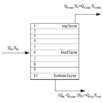
Figure 8‑6 - Layered Flotation Model
The model is based on the solids flux concept: a mass balance is performed around each layer, providing for the simulation of the solids profile throughout the DAF unit under both steady-state and dynamic conditions.
The model is based on traditional solids flux analysis, with an additional component for flotation. Model detail is provided in the previous section of this chapter devoted to one-dimensional sedimentation models.
The solids flux due to the bulk movement of the liquid is calculated by multiplying the solids concentration by the liquid bulk velocity (flow divided by area), which may be up or down depending on the position relative to the feed layer.
The solids flux due to flotation is specified by the same double exponential function used for sedimentation (Equation 8.1). The parameters within Equation 8.1 are altered to account for effects of flotation:
vsj = floating velocity in layer j (m/d)
vmax = floating velocity with optimal air-to-solids ration (m/d)
rhin = hindered zone floating parameter (m3/gTSS)
rflo = free floating zone floating parameter (m3/gTSS)
X jo = Xj – Xmin, where Xmin is the minimum attainable suspended solids concentration, Xj is the suspended solids concentration in layer j
The minimum attainable solids concentration in a layer, Xmin, is calculated as a fraction (non-floatable fraction of fns) of the influent solids concentration to the DAF unit:
Equation 8.6
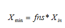
It is subject to a maximum value specified by the user, the maximum non-floatable solids or Xminmax. The floating velocity is lower bounded to zero, so that if the user specifies parameter values that would result in floating velocities becoming negative, a warning message is printed in the simulation Log window. The floating velocity is also subject to a maximum value specified by the user, the maximum floating velocityor vbnd.
This section of the chapter contains a description of the various model parameters and inputs that the user encounters when using the flotation model.
These menu items are found under the Parameters sub-menu item Physical. This input form contains the actual physical dimensions of the DAF unit being modelled, including the tank surface area, the maximum water level or height of the tank, and the location of the feed point relative to the bottom of the tank. The fourth item on the form allows the user to define the number of equivalent layers contained within the model. The physical parameter form is shown in Figure 8‑7.
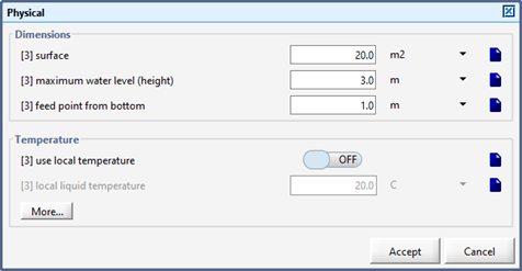
Figure 8‑7 – Physical Parameters for the DAF Unit
The operational parameters for the DAF unit are located within the Parameters sub-menu item Operational. This input form contains the polymer dosage (g polymer/kg solids) and the air-to-solids ratio (g air/g solids) for daily operation of the DAF unit. The maximum float flow is an upper boundary limit for the amount of float that can be removed from the DAF unit. The operational input form is shown in Figure 8‑8.
Under the sub-heading other parameters, the optimal polymer dosage and optimal air-to-solids ratio are defined. These two values provide an estimate of the best expected solids condition. The optimal values may be expressed based on past operating experience with the actual DAF unit or may be provided through manufacturer literature. The dry material content of the float at the optimal polymer dosage is defined as a percentage. The dry material content of the float without polymer dosage is also defined. The model will use the range between these two values to predict the dry material content of the float under actual operating conditions.
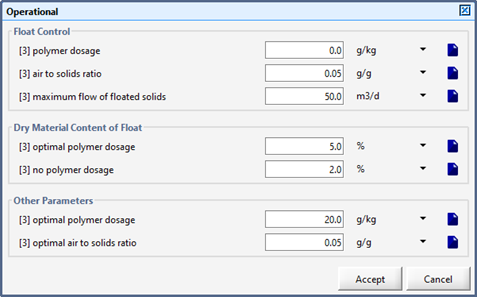
Figure 8‑8 - Operational Parameters for the DAF Unit
The Flotation parameters, shown in Figure 8‑9, are used to define the variables contained within the model (Equation 8.1). The maximum floating velocity provides an upper boundary limit for the model. The next variable is the expected floating velocity under the optimal air-to-solids ratio, as defined under the operational input form. The hindered zone and free floating zone floating parameters control the floating velocity defined in Equation 8.1. There will likely be a fraction of solids, which cannot be removed by flotation. This fraction is characterized as the non‑floatable fractionand an upper boundary for this parameter as a concentration is set as the maximum non-floatable solids.
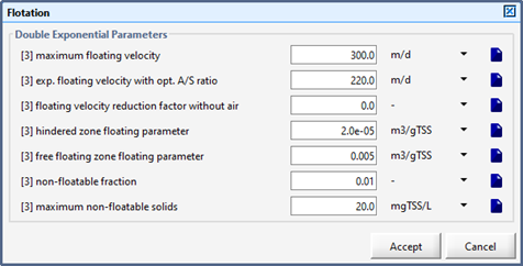
Figure 8‑9 – Flotation Parameters for the DAF Unit
This chapter describes the deep bed granular filtration models available in GPS-X. The continuous and massbalance models are based on empirical removal efficiencies. The simple1d model is a mechanistic model based on continuity and kinetic equations that describe the removal of suspended particles by deep bed granular filters.
The basis for the continuous model is the direct specification of the filter performance through two parameters: the backwash flow fraction and the backwash solids mass fraction (Figure 9‑1). The backwashout connection (bottom left of object) is not used in this model.
The backwash flow fraction (frqbw) is the fraction of the incoming flow to the filter (input connection - top left of object) that is used for backwash. Using this parameter, GPS-X will calculate a continuous backwash flow (Qb) associated with the backwashout stream (top right of the object):
Equation 9.1
![]()
The continuous output flow (bottom right of the object), is then calculated from the difference between the input flow and the backwash flow:
Equation 9.2
![]()
The backwash solids mass fraction (frxbw) is the fraction of incoming solids that is captured by the filter, ending up in the backwash stream. Using this parameter, GPS-X calculates the solids concentration in the backwash stream (Xb):
Equation 9.3
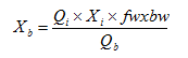
The solids concentration in the output stream (Xo) is calculated from:
Equation 9.4
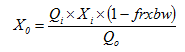
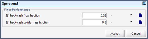
Figure 9‑1 – Operational Parameters Form – Continuous Model
The massbalance model is based on empirical removal efficiency for suspended solids, BOD and TKN parameters. A `best' value is set for removal efficiency immediately after backwash. The removal efficiency decreases during the filter cycle time as the filter is fouled until the next backwash. The decrease in the removal efficiency is modelled with an exponential function:
Equation 9.5
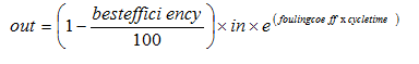
where:
out = filter effluent component concentration (mg/L)
in = filter influent component concentration (mg/L)
bestefficiency = best removal efficiency after backwash (%)
foulingcoeff = fouling coefficient
cycletime = time elapsed since last backwash (h)
A minimum efficiency value for suspended solids removal is also defined as an operational parameter. This parameter does not affect removal computed by the model but warns the user that, once removal of solids gets below this minimum value, the filter is undergoing high headloss.
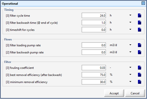
Figure 9‑2 – Operational Parameters Form – Massbalance Model
The massbalance model accounts for the mass accumulated in the filter during the filter cycle time. The accumulated mass is removed during backwash. Therefore, stoichiometric parameters for the filter effluent and the backwash may be specified. The operational parameters for the massbalance model are shown in Figure 9‑2.
The basis for the simple1d model is the combination of the continuity (mass balance) and the kinetic partial differential equations by Horner et al. (1986), which describe the removal of suspended particles by a granular filter:
Equation 9.6
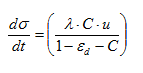
where:
s = volume of deposited solids per unit bed volume
C = concentration of suspended particles at depth L and time t
u = approach velocity (velocity of the fluid above the filter bed)
ed = porosity of deposited solids
When combined with defining equations for the deposited (attached) solids (X= s×d) and the unattached solids (X = C ×dd) in the filter, the following equation is derived for the simple 1d model:
Equation 9.7
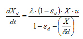
where:
X = unattached solids
Xd = attached (deposited) solids
δd = density
The filter bed is divided into layers and it is assumed that the specific deposit is uniform across each layer. During the backwash cycle, the average deposit through all layers of the filter is used. The average deposit after backwash is used as the initial condition for the subsequent filter run.
This section discusses the various model parameters and inputs that the user encounters when using the simple1d model.
These menu items are found under the Parameters sub-menu item Physical and contain both real physical dimensions to describe the actual filter modelled, and model dimensions which allow the user to specify the number of layers and an effective particle diameter. The real dimensions of the filter are the bed surface area and the bed depth.
Operational items, found under the Parameters sub-menu, include the basis for the duration of the filtration run. The duration of the filtration run may be based on a user-specified time, headloss or effluent suspended solids concentration. The filtration run may also be set manually. Other operational parameters include the influent flow and specification of the backwash parameters (duration, rate).
The stoichiometric fractions available for the model are the ratios of particulate COD to VSS, VSS to TSS and BOD5 to BODultimate.
The filtration constants required for the model are shown in Figure 9‑3. The filtration constants include the clean bed filtration coefficient (lo), the initial porosity of the filter bed (eo) and the porosity of deposited solids (ed), the ultimate bulk specific deposit (su), and the density and dry material content of the solids. The packing factor is used in the defining equation for the variation of the filtration coefficient with the bulk specific deposit as given by Ojha and Graham (1992).
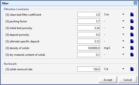
Figure 9‑3 - Filter Parameters
The flow and
characteristics of the filter flow and backwash can be displayed on
output graphs. There are various filter variables available in the
sub-menus under Output Variables. The output variables
include dilution, headloss and rates, the
unattached and attached solids in the filter and
filter conditions (i.e. bulk deposit, bed porosity).
This chapter describes the aerobic and anaerobic digestion models used in GPS-X.
This section describes the basic anaerobic digestion model associated with the anaerobic digester object. It is a modified version of the model developed by Andrews (1969), and Andrews et al. (1971). The modifications to the original model are:
· The addition of temperature sensitivity for the hydrolysis of volatile suspended solids (VSS) and the growth of methanogenic organisms. The Arrhenius equation is used with a base temperature of 35 degrees Celsius.
· The chemical equilibria were modified by introducing Hydromantis' pH model (See PH Tool section in CHAPTER 12).
· The introduction of particulate inert inorganic material (xii). This component remains unchanged within the digester and is introduced for the sole purpose of assessing its impact on other processes downstream of the digester.
· The addition of a rate for toxic substance degradation.
The basic anaerobic digestion model consists of two reactors: one for the liquid phase and the other for the gaseous phase. Both are modelled as completely mixed reactors. Transfer of gaseous products between the liquid phase and the gaseous phase is modelled using a standard two-film mass transfer equation. Gaseous carbon dioxide (CO2) and methane (CH4) are assumed to follow the ideal gas law. No further reactions take place in the gaseous phase, which has a total gas pressure of 760 mm of Hg (i.e., atmospheric pressure).
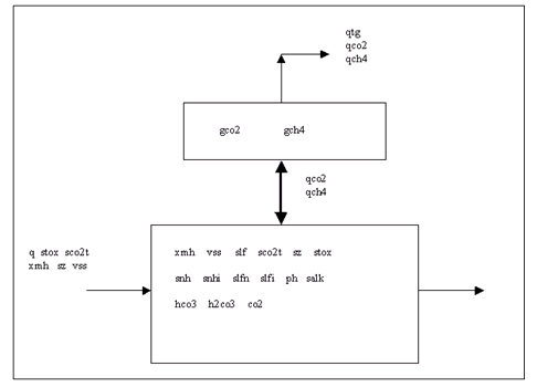
Figure 10‑1 - Schematic Diagram of the Anaerobic Digestion Model
A schematic diagram of the anaerobic digestion process is shown in Figure 10‑1, where:
qtg: = total gas flow (m 3/d)
qco2 = CO2 gas flow (m 3/d)
qch4: = CH4 gas flow (m 3/d)
gco2: = partial pressure of CO2 (atm)
gch4 = partial pressure of CH4 (atm)
State Variables
xmh: = methanogens (gCOD/m3)
vss = volatile suspended solids (gCOD/m 3)
slf = total volatile fatty acids (gCOD/m3)
sco2t = total soluble CO2(moles/L)
sz = net cations (moles/L)
stox = toxic substance (g/m3)
Composite Variables
snhn = free ammonia (moles/L)
snhi = ionized ammonium (moles/L)
slfn = non-ionized volatile fatty acids (moles/L)
slfi = ionized volatile fatty acids (moles/L)
pH = pH
hco3 = bicarbonate (moles/L)
h2co3 = carbonic acid (moles/L)
salk = alkalinity (g/m3)
The mathematical equations used in the liquid and gaseous phases are provided in the corresponding Model matrix form in Appendix A. The general reaction pathway is shown in Figure 10‑2.
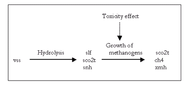
Figure 10‑2- General Reaction Pathway
The relative amounts of chemical components produced by the biological and chemical reactions in the anaerobic digester are specified by stoichiometric coefficients. The chemical reaction stoichiometry is defined by the balanced chemical reaction equations. The biological stoichiometry is defined by the yield coefficients.
Seven yield coefficients are used by the basic model:
ya = slf / vss
yc = xmh / slf
ye = gch4 / xmh
yg = xmh / snhi
In each case the yield is defined as the ratio of the change in a product to the change in a reactant. Volatile acids and volatile suspended solids are expressed as their equivalent chemical oxygen demand (COD).
Volatile Suspended Solids
The rate of hydrolysis of VSS is assumed to be first order with respect to the concentration of VSS. A temperature correction factor (ftkco) is calculated using the Arrhenius equation with a base temperature of 35 degrees Celsius. The temperature correction factor is incorporated in the equation for the hydrolysis rate:
Equation 10.1
![]()
where:
kco = rate constant for the hydrolysis of VSS
Methanogenic Organisms
The growth of the microorganisms responsible for the generation of methane is modelled using the Monod equation modified by switching functions (similar to the IWA models). The rate of growth of methane producing bacteria (r2) is assumed to be proportional to their concentration (mumh). The model uses un‑ionized volatile acids (slfn) as the substrate and incorporates two switching functions for inhibition: one for inhibition by slfn and the other by free ammonia (snh).
The resulting rate equation is:
Equation 10.2
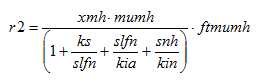
where:
ftmum = the temperature correction factor for the growth of methanogens
mumh = maximum specific growth rate for methanogens
ks = the half-saturation coefficient
kia, kin = the inhibition constants for slfn and snh, respectively
As in other biological models, the rate of decay of methane producing bacteria (r3) is assumed to be proportional to their concentration:
Equation 10.3
![]()
where:
kd = the decay rate coefficient
The effect of toxic substances (stox, input as a special component to the influent parameters) is taken into account by using a first order expression for the rate of inactivation of methane bacteria:
Equation 10.4
![]()
where:
ktox = the inactivation rate coefficient
Based on the above rates, the net rate of generation of methanogens (rxmh) is:
Equation 10.5
![]()
Toxic Substances
A rate of toxic substance degradation (r5) is incorporated in the basic model. The rate of degradation is assumed to be first order with respect to the concentration of toxic substances:
Equation 10.6
![]()
where:
kb = toxic substance degradation rate
Total Volatile Fatty Acids
The kinetic expression for total volatile fatty acids (slf) can be established using the previously presented kinetic expressions and appropriate yield coefficients:
Equation 10.7
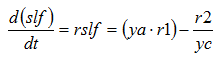
where:
(ya r1) = rate of generation of slf by hydrolysis
‑r2/yc = rate of utilization of slf by the growth of methanogens
Methane
The biological generation of methane can be expressed in terms of bacterial growth rates and yield coefficients. The model assumes that the solubility of methane is negligible and all methane generated is immediately transferred to the gas phase:
Equation 10.8
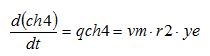
where:
vm = volume of the liquid phase in the digester
Carbon Dioxide
The mass transfer of carbon dioxide between the liquid and gas phases is calculated using the standard two-film gas transfer equation.
Equation 10.9
![]()
where:
klac2o2 = mass transfer coefficient for CO2
co2sat = saturation concentration of CO2 in the liquid phase, and H2co3=sco2t-hco3-co2
The pH model within the basic digester model calculates bicarbonate (hco3) and carbonate (co2). The concentration of dissolved CO2 in the liquid phase at equilibrium (co2sat) is calculated using Henry's law:
Equation 10.10
![]()
where:
henryco2 = Henry’s law constant for CO2
gco2 = partial pressure of CO2 in the gas phase
Combining the above equations:
Equation 10.11
![]()
The rate of biological generation of total soluble carbon dioxide (rsco2t) can be expressed in terms of bacterial growth rates and yield coefficients. Combined with the above equation results in the total reaction rate for dissolved CO2 (rsco2):
Equation 10.12
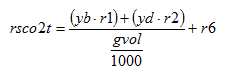
where:
(yb r1) = rate of generation of sco2t by the hydrolysis of vss
(yd r2) = rate of generation of sco2t by the growth of methanogens
gvol = gas constant for CO2 in L/mole
The mass transfer of CO2 between the liquid and gas phases (r6) is negative when CO2 is transferred from the liquid to the gas phase.
Ammonia
Ammonia (snh) is assumed to be produced only at the hydrolysis/acidification stage. Ammonia (snh) is utilized by the methanogenic organisms for growth. The rate of generation of free ammonia (rsnh) is modelled as:
Equation 10.13
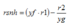
where:
(yf r1) = rate of generation of ammonia by hydrolysis/acidification
-r2/yg = rate of consumption of ammonia due to growth of methanogenic organisms.
The chemical equilibria and the pH calculation used for ammonia (snh) and ammonium ion (snhi) are based on Hydromantis' pH Model..
This section of the chapter discusses the various model parameters and inputs that the user would encounter when using this model. The Parameters menu is shown in Figure 10‑3

Figure 10‑3 – Parameters Menu for the Anaerobic Digester
The physical parameters for the Mantis2 digester model are the volume of the liquid phase or maximum volume (vm), the effective volume fraction (effvol), the headspace volume (vgas), the total gas pressure (itpcon), and the digester temperature (temp). The effective volume fraction accounts for differences in the designed and actual digester volume (due to mixing, inert solids, precipitation, etc).
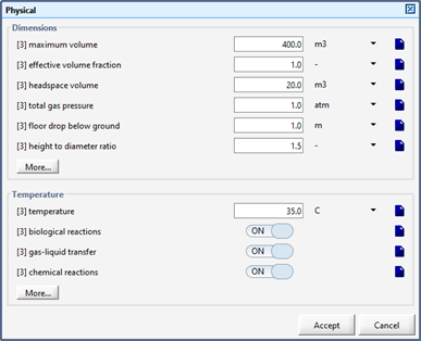
Figure 10‑4 - Physical Parameters
The Operational parameters shown in Figure 10‑5 are exclusively related to the control of the pumped flow. These parameters are similar to the control parameters used in other models (e.g., CSTR reactor).
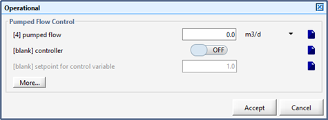
Figure 10‑5 –Operational Parameters
These menu items are found under Parameters sub-menu items Influent and Effluent.
The Influent sub-menu, shown in Figure 10‑6, allows the user to define influent parameters that are exclusive to the basic digester model: soluble total CO2 (sco2t), toxic substance concentration (stox), methanogens concentration (xmh) and net cations (strong bases)(sz).
The Effluent sub-menu, shown in Figure 10‑7, allows the user to define special components to the effluent of the anaerobic digester: inert soluble COD (si) and the fraction of the effluent VSS that is inert (frinert).
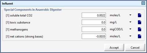
Figure 10‑6 - Influent Parameters (Basic Digester Model)
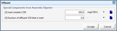
Figure 10‑7 – Effluent Parameters (Basic Digester Model)
These parameters, found under the Parameters sub-menu item pH Solver Set up (Figure 10‑8) define the initial pH value (ph), the pH boundaries: minimum (lowph), and maximum (highph) values, and the required pH accuracy (errorph). Parameters for the search routine of the pH are presented in this sub-menu.
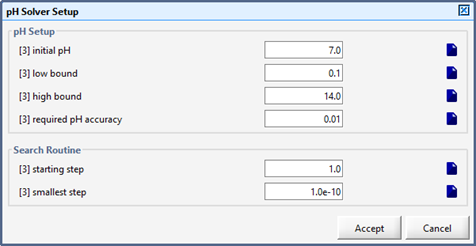
Figure 10‑8 - pH Solver Set up
The kinetic parameters (shown in Figure 10‑9) are found under Parameters sub-menu item kinetic. The maximum specific growth rate for methanogens (mumh) and the rate constant for hydrolysis of vss (kco) are defined for 35 degrees Celsius and corrected by the model using the Arrhenius equation with the temperature coefficients indicated at the bottom of this menu (tmumh & tkco). The rest of the kinetic parameters in the basic model are not temperature-dependent.
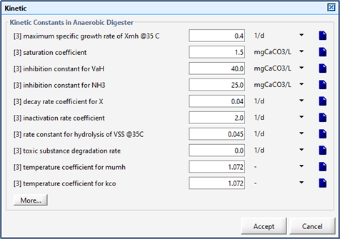
Figure 10‑9 - Kinetic Parameters
The stoichiometric parameters (Figure 10‑10) are found under Parameters sub-menu item Stoichiometric. The first set of stoichiometric parameters consists of conversion factors: particulate COD (xcod) to vss ratio (icvcon), BOD5 (bod) to BOD ultimate (bodu) ratio (fbodcon).
Conversion factors that are unique to the digester basic model are the mass acetic acid to COD factor(ac2cod), the molecular weight of fatty acids (mwfat) and the gas constant (gvol).
Using these factors and the parameters defined in the Effluent sub-menu, the basic digester model establishes the values for the composite parameters. These parameters will modify the stoichiometry of the effluent stream.
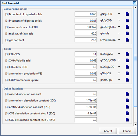
Figure 10‑10 - Stoichiometric Parameters
The second set of stoichiometric parameters consists of yields. The relative amounts of chemical components produced by the biological reactions in the anaerobic digester are specified by these yields.
Other stoichiometric parameters in this sub-menu are the dissociation constants used to calculate the ionized components in the pH model incorporated in the basic model. The dissociation constant for ammonium (kncon) is defined for 20 degrees Celsius and is temperature sensitive, i.e., the model corrects it for temperature changes using the following equation:
Equation 10.14
![]()
The rest of the dissociation constants are not corrected for temperature changes in the basic model.
Gas transfer parameters are also defined on this form. The mass transfer coefficient for carbon dioxide gas (sco2) between the liquid and gas phases (KLaco2) is not corrected by temperature in the basic model. Henry's law constant for carbon dioxide (henryco2) is also included in this item and is not corrected for temperature.
Anaerobic Digestion Model #1 (ADM1) (Batstone et al., 2002) is implemented in GPS-X according to the ADM1 COST Benchmark (Rosen and Jeppsson, 2002), with the following changes:
· Several differential equations that describe the acid-base equilibrium of the system (equations for Sva-, Sbu-, Spro-, Sac-, Shco3-, and Snh3) have been converted to algebraic equations as described in Table B.3 of Batstone et al. (2002). These processes are very fast and contribute to the stiffness of the system of differential equations.
· The differential equation for Sh2 has been converted to an algebraic equation to improve the simulation speed. This process is very fast and contributes to the stiffness of the system of differential equations. This approach is described by Rosen et al. (2005).
These changes substantially increase the solution speed of ADM1 in
GPS-X and allow an integration algorithm other than Gear’s Stiff to
be used. Double Precision arithmetic should be used when
solving ADM1 in GPS-X
(accessed in
Options > Preferences > Build
tab)
The structured model includes five process steps including disintegration, hydrolysis, acidogenesis, acetogenesis and methanogenesis. The model uses 32 dynamic state variables, 6 acid-base kinetic processes, 19 biochemical processes, and 3 gas-liquid transfer processes.
A simplified ADM1 material flow diagram is shown in Figure 10‑11. For a full description of the model, the reader is referred to Batstone et al,. (2002). Implementation details are found in Rosen and Jeppsson (2002).
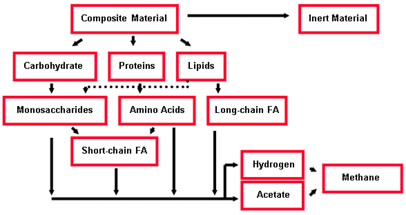
Figure 10‑11 - Simplified ADM1 Material Flow Design
In GPS-X, the ADM1 model makes use of an ASM1 to ADM1 interface developed by Copp et al. (2003). This interface allows ADM1 to be used within a full-plant layout that uses ASM1 to model activated sludge processes.
When using ADM1 there are two possible scenarios:
· The influent stream is represented by an influent object. This case is more difficult and requires that you specify the influent in the influent object and in the Influent Form in the digester object. See Figure 10‑12 for a graphical description of this procedure. The section entitled “ADM1 Model Set up Suggestions” gives suggestions on how to characterize the influent.
· The influent stream is an output stream from another object. This case is simpler as the object that precedes the digester will take care of the characterization of the stream itself. The user still needs to specify the parameters found in the Influent form of the digester object. See Figure 10‑13 for a graphical description of this procedure. The section entitled “ADM1 Model Set up Suggestions” gives suggestions on how to characterize the influent.
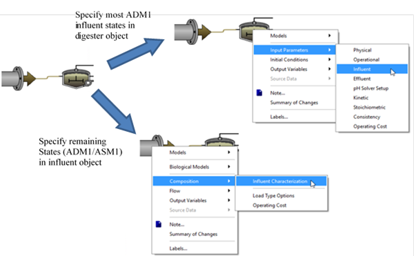
Figure 10‑12 - Method of Specifying the ADM1 Influent when the Influent Stream is Represented by an Influent Object
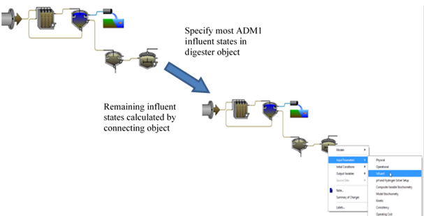
Figure 10‑13 - Method of Specifying the ADM1 Influent when the Influent Stream is an Output Stream from another Object
The following hints are useful for characterizing influent streams to a digester object using the ADM1 model. Because the ADM1 model uses a different set of state variables than the ASM activated sludge models, supplementary information has to be supplied for the ASM1/ADM1 interface.
In typical simulation practice, you will not have all the information you need, and will have to estimate the values for many of the ADM1 influent parameters. These guidelines can be useful for making sure that the estimates are used correctly. The following suggestions are for the Carbon-Nitrogen Library (CNLIB).
Table 10‑1 – ADM1 State Variables Set on the ADM1 “Influent” Parameter Menu
|
Parameter |
Suggestion |
|
cations |
Must be measured or estimated or can be set to the value of the Sic (inorganic carbon) state in ADM1. |
|
anions |
Must be measured or estimated or can be set to the value of the Sin (inorganic nitrogen) state in ADM1. |
|
long chain fatty acids |
Must be measured or estimated. It is part of Ss in the influent object form. |
|
total valerate
|
Must be measured or estimated. It is part of Ss in the influent object form. |
|
total butyrate |
Must be measured or estimated. It is part of Ss in the influent object form. |
|
total propionate |
Must be measured or estimated. It is part of Ss in the influent object form. |
|
total acetate |
Must be measured or estimated. It is part of Ss in the influent object form. |
|
hydrogen gas |
Set to zero |
|
methane gas |
Set to zero |
|
proteins |
Must be measured or estimated. It is part of Xs in the influent object form. |
|
sugar degraders |
Set to zero |
|
amino acid degraders |
Set to zero |
|
long chain fatty acid degraders |
Set to zero |
|
valerate and butyrate degraders |
Set to zero |
|
propionate degraders |
Set to zero |
|
acetate degraders |
Set to zero |
|
hydrogen degraders |
Set to zero |
When the influent stream is represented by an influent object, the states influent model should be used in the influent object. Some of the states are ADM1 states and these need to be estimated. Some states are not relevant for ADM1 and can be ignored. Some states form a fraction of an ADM1 state and when added up need to correspond to the values entered into the influent form of the ADM1 object. More detailed descriptions are given below:
Table 10‑2 – ADM1 State Variables Set in the Influent Object
|
Parameter |
Suggestion |
|
inert inorganic suspended solids |
Must be measured or estimated. It is not an ADM1 state but will impact the solids concentration. |
|
soluble inert organic material |
Same as the Si state in ADM1 |
|
readily biodegradable substrate |
Sum of Monosaccharides, Amino acids, Long chain fatty acids, Total valerate, Total butyrate, Total propionate, Total acetate, and Carbohydrates states in ADM1. Make sure this value is the sum of the values entered for these states in the ADM1 influent stream. |
|
particulate inert organic material |
Same as Xi state in ADM1. |
|
slowly biodegradable substrate |
Sum of composites, proteins, and lipids states in ADM1. Make sure this value is the sum of the values entered for these states in the ADM1 influent stream. |
|
active heterotrophic biomass |
Set to zero unless you have an estimate of it. |
|
active autotrophic biomass |
Set to zero unless you have an estimate of it. |
|
unbiodegradable particulates from cell decay |
Becomes part of Xi state in ADM1. Unless you know Xu, use Xi above and set this to zero |
|
internal cell storage product |
Not used. |
|
dissolved oxygen |
Not in ADM1 but used by GPS-X to estimate the COD demand of the influent stream. It is assumed that both oxygen and nitrate will be reduced instantaneously upon entering the anaerobic environment, so the total incoming COD is reduced by this incoming COD demand to compensate for the reduction of the electron acceptors present in the incoming stream. |
|
free and ionized ammonia |
Sin state in ADM1 (inorganic nitrogen). Make sure that correct units are used. |
|
soluble biodegradable organic nitrogen |
(nitrogen
faction in amino acids = 0.098) |
|
particulate biodegradable organic nitrogen |
Use the following formulas:
Xnd = total TKN - Snd - Snh - inxu*Xu -inxi*Xi
total TKN = Sin +
Ni
where:
Snd = conc. of soluble biodegradable organic nitrogen Snh = conc. of free and ionized ammonia inxu = nitrogen fraction of unbiodegradable particulates from cell decay (0.068 in Mantis, 0.06 in ASM1) inxi = nitrogen fraction of particulate inerts (0.068 in Mantis, 0.06 in ASM1) Xu = conc. of unbiodegradable particulates from cell decay Ni = nitrogen fraction of Si and Xi Si = conc. of soluble inerts Xi = conc. of particulate inerts Naa = nitrogen fraction of amino acids (0.098) Saa = conc. of amino acids Nxc = nitrogen fraction of composites (0.0376) Xc = conc. of composites |
|
nitrate and nitrite |
Not in ADM1 but used by GPS-X to estimate the COD demand of the influent stream. It is assumed that both oxygen and nitrate will be reduced instantaneously upon entering the anaerobic environment, so the total incoming COD is reduced by this incoming COD demand to compensate for the reduction of the electron acceptors present in the incoming stream. |
|
dinitrogen |
Set to zero. |
|
alkalinity |
Sic state in ADM1 (inorganic carbon). |
The objective of the aerobic digestion process is to stabilize and reduce the mass of solids for disposal. In this process, microorganisms consume their own protoplasm for energy; they are assumed to be in the endogenous phase. This phase is accounted for in the biological models associated with the CSTR object, but in aerobic digestion, destruction of particulate inert organic material also occurs.
The models associated with the aerobic digester are given the name <model>dig, where <model> is the associated activated sludge model (such as asm1, etc.). The only difference between the activated sludge model and its corresponding aerobic digester model is an added first-order reaction. This additional reaction adjusts the particulate inert organic concentration to account for the destruction of the inert organics:
Equation 10.15
![]()
where:
rxi = rate of reaction for particulate inert organics (xi) (under Parameters – Kinetics menu of the anaerobic digester object)
ki = inert bioconversion rate
No loss of COD is involved in this process, and no electron acceptor is utilized. This destruction process converts particulate inert organics (xi) to slowly biodegradable substrate (xs). The slowly biodegradable substrate formed is then hydrolyzed, releasing an equivalent amount of readily biodegradable COD.
The UASB/EGSB model is available only in MANTIS2LIB. The Mantis2 model is used to model the biological-chemical reactions in the reactor. Some of the assumptions made in the development of model are listed below.
1. The hydraulic regime in the UASB/EGSB is modeled as completely mixed reactor.
2. The substrate diffusion into the granule is assumed to be not limiting and the reactions are modeled similar to the suspended growth systems.
3. The average granule properties are used to estimate the granule settling velocity and bed expansion in the reactor.
4. A semi-empirical model is used to estimate the solid concentration distribution above the bed.
The simplified model structure is a first attempt to dynamically model the UASB//EGSB reactors for practical engineering problems.
Some of the important inputs and outputs of the model are described in following sections.
Additional sets of input parameters are required for the UASB/EGSB model to estimate the granule settling velocity, bed fluidization and solid distribution profile above the sludge bed.
The Reactor Parameters can be accessed from the Input Parameters menu item (Figure 10‑14). The Reactor Parameters form is as shown in Figure 10‑15.
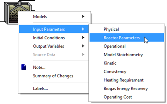
Figure 10‑14 - Reactor Parameters for UASB/EGSB Reactor
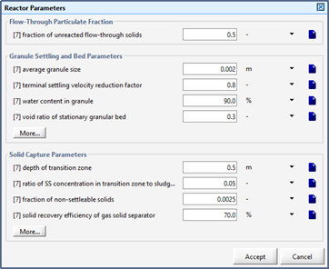
Figure 10‑15 - Reactor Parameters Input Form
Fraction of un-reacted flow-through solids
It is well known that UASB/EGSB reactors are not very effective in treating the suspended solids in the wastewater. A fraction of the solids in the influent stream may just flow through the UASB/EGSB reactor without getting adsorbed or reacted in the reactor. This parameter allows users to specify the fraction of solids which will pass through the reactors un-reacted. Although, this phenomenon is normally observed, it is not very well quantified. The default value of this parameter is set at 0.5. In actual situation, depending on the bed expansion, the value of this parameter may vary.
Average granule size
This parameter is used to calculate the settling velocity of the granules in the granular bed. The estimated settling velocity is also used in estimating the bed expansion in the reactor. A default value of 2mm is used.
Terminal velocity reduction factor
The observed settling velocity of the biological granules is found to be less than the settling velocity estimation procedures. Normally a reduction factor of 0.7-0.8 is suggested in the literature.
Water content in granule
This parameter defines the water content in a granule and is used to estimate the density of the granule required in the settling velocity estimation procedure.
Void ratio of stationary granular bed
This parameter defines the void volume in the granular bed under no flow conditions.
Depth of transition zone
The UASB/EGSB model uses a semi-empirical model to decide the solid profile above the expanded granule bed. In the present model it is assumed that there exists a transition zone above the sludge bed in which the solid concentration changes from the concentration in the bed to a fraction of concentration at the end of transition zone. The depth of this transition zone will affect the solid profile and solid capture efficiency in the reactor.
Ratio of SS in transition zone to sludge bed
As described above, this parameter represents the ratio of solid concentration at the transition zone boundary to the solid concentration in the granule bed.
Fraction of non-settleable solids
This parameter signifies the fraction of finer particles in the bed which are non-settleable. This ratio is expressed with respect to the solid concentration in the reactor.
Solid recovery efficiency of gas solid separator
The solid distribution curve above the granule bed is used to estimate the solids concentration reaching the gas solid separator at the top UASB/EGSB reactors. Depending on the efficiency of the gas solid separator the concentration of solids escaping in effluent is estimated.
The proportional splitters in GPS-X can be set up for constant flow split, variable split based on a timer, or variable split based on flow. In the Parameters > Splitter Set up form you can select the appropriate splitting mode. They are described below:
When using this splitting mode, the split fractions do not change (as entered under the Constant section), or are read from a file, or are controlled by any other method (controller tool or customization).
When using this splitting mode, the split fractions, as entered under the Constant section, will be rotated through the connection points according to the specified time interval.
When using this splitting mode, the split fractions, as entered under the Constant section, will be rotated through the connection points according to the specified volume. Once the specified volume has passed through the splitter input, the fractions will be moved to the next output connection.
A typical example of using this functionality is a multiple train SBR plant, where the influent has to be sent to a different SBR tank either by timer control or by discharged volume.
A control splitter can be used to split flow into a set flow rate and an overflow. This object is useful for setting flow bypass controls.
The pumped flow rate is set in the Parameters > Pumped Flow menu. If the incoming flow is equal to or less than the pumped flow rate, all of the flow will exit through the pump connection point. If the incoming flow is greater than the pumped flow rate, the excess flow will exit through the overflow connection point.
An automatic PID controller can be used in this object to control another variable in GPS-X with the pumped flow rate.
The noreact model for Pumping Station allows user to use continuous or intermittent pumping based on height or volume based control.
The input form is as shown in Figure 11‑1:
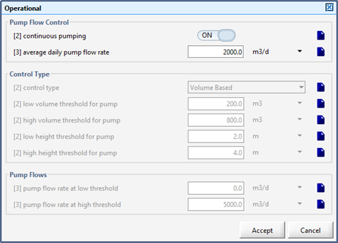
Figure 11‑1 - Pumping Station Menu
Continuous pumping - this variable controls whether continuous pumping or intermittent pumping is used.
Average daily pump flow rate - this flow rate is used for continuous pumping rate and also in the calculation of steady state calculations when intermittent pumping is selected.
Control Type - the option gets activated when continuous pumping is OFF. User may select from volume or height based control options.
Low volume threshold for pump - this variable defines the volume in the tank below which the pump operates at low threshold pumping capacity. The option is activated when Volume Based control is selected.
High volume threshold for pump - this variable defines the volume in the tank above which the pump operates at maximum threshold pumping capacity. The option is activated when Volume Based control is selected.
Low height threshold for pump - this variable defines the height in the tank below which the pump operates at low threshold pumping capacity. The option is activated when Height Based control is selected.
High height threshold for pump - this variable defines the height in the tank above which the pump operates at maximum threshold pumping capacity. The option is activated when Height Based control is selected.
Minimum pump capacity - this is the capacity at which the pump operates when the volume in the tank is below the low volume. The option is activated when continuous pumping is OFF.
Maximum pump capacity - this is the capacity at which the pump operates when the volume in the tank is above the high volume. The option is activated when continuous pumping is OFF.
One model is available for this object (empiric).
In this zero-volume model, the soluble state variables are not affected, but solids are partitioned into one of two streams based on a user-defined solids separation factor. Flow can be pumped from either of the effluent connection pipes and the difference between the pumped flow and influent flow is diverted to the other effluent connection. Solids concentrations in the two effluent streams are calculated through a mass balance based on flows and the separation factor. An example calculation is given below:
|
Influent Flow |
= |
100 m3/d |
|
Influent xbh |
= |
1000 g/m3 |
|
|
|
|
|
Mass Influent xbh |
= |
100 x 100 = 100,000 g/d |
|
|
|
|
|
Pumped Flow (user-defined) |
= |
10 m3/d – concentrate |
|
Filter Efficiency (user-defined) |
= |
0.90 |
|
|
|
|
|
Filtrate Flow |
= |
90 m3/d |
|
Filtrate xbh Concentration |
= |
100 g/m3 |
|
Filtrate xbh Mass |
= |
90 x 100 = 9,000 g/d |
|
|
|
|
|
Concentrate xbh Mass |
= |
100,000 – 9,000 = 91,000 g/d |
|
Concentrate xbh Concentration |
= |
91,000 / 10 = 9,100 g/m3 |
In the nonreactive noreact model, the effect of dilution on wastewater components is described, but all reaction rates are set to zero (no biological reactions are occurring). The tank has aeration terms (for modelling of pre-aeration) and a built-in pump, and both aeration and pumped flow can be controlled with feedback controllers (P, PI, PID) analogous to the ones found in aeration tanks and settler/clarifier objects.
This model can be used to simulate an equalization tank either off-line or in-line, as the volume is variable. In an off-line or variable volume mode (flow equalization), the pump connection should be used with the proper controller set up, while for concentration equalization in fixed volume tanks the overflow connection is best used.
Reactions can be added by double-selecting the model (noreact) and editing the rate equations of the individual components.
In a sludge pretreatment process, the particulate organic compounds are converted into soluble organic compounds. The degree of solubilization normally depends on the intensity of the treatment. There are many different types of sludge pre-treatment processes. These processes can mainly be divided into thermal, mechanical and chemical treatment. Thermal, mechanical disintegration, ultrasound, microwave, alkaline treatment ozonation, Fenton etc. are some of the treatment which have been normally applied. For thermal and mechanical treatments, the main operational parameter affecting the degree of solubilization is the specific energy input, while for chemical treatment it is the specific chemical dose. The specific energy input and specific chemical dose are normally expressed in terms of per unit of solids. As the mechanisms in sludge pretreatment processes are normally too complex to describe through a mechanistic model, empirical approach of modelling is normally adopted. For general engineering purpose, this approach is sufficient to evaluate different options and help in decision making.
The general sludge pre-treatment process model in GPS-X includes the following transformations.
1. The model describes the relationship between degree of solubilization to the operational parameters like specific energy input or specific chemical dose using a solubilization saturation curve.
2. The model allows conversion of the non-biodegradable organics into biodegradable organics.
3. The model allows for loss of during the treatment
The sludge pretreatment model is available in MANTIS2LIB. Three main transformations are described in the model.
1. Inactivation of bacterial biomass
The sludge pre-treatment normally results in bacterial inactivation. The bacterial inactivation may happen due to disintegration of the cell wall and release of soluble organic products. The biological inactivation will results in production of soluble and particulate organic products. Depending on the nature of treatment as part of the COD may be lost due to oxidation.
2. Conversion of Inert Organics (Xi and Xu)
The inert particulate COD is reduced during the sludge pre-treatment. A part of the particulate inert COD is assumed to convert to the slowly biodegradable COD. The particulate inert COD also solubilize and results in soluble biodegradable and soluble inert COD. Depending on the treatment a part of the inert organic COD may be lost.
3. Conversion of slowly biodegradable COD (Xs)
The particulate slowly and very slowly biodegradable COD is solubilized and results in the soluble biodegradable substrate.
The implemented model is an input-output model in which all the input states are instantaneously converted to the output states. It is assumed that the retention time in the chemical-mechanical disintegration reactors are small.
The In-line Chemical Dosage object (Figure 11‑2) can be used to simulate chemical addition for soluble phosphorus removal and coagulation/flocculation of soluble and colloidal components. Two chemical precipitation models chemeq and metaladd are available in GPS-X. The metaladd model is available in all the libraries having soluble phosphorus as a state variable. The chemeq model is not available in MANTIS2LIB. The metaladd model considers the effect of pH and solubility product in the metal precipitation reactions.
Figure 11‑2 - In-line Chemical Dosage Object
The P-removal model is available only in the CNP library. The model is based on the stoichiometry of the chemical precipitation of soluble phosphorus. The model is set up to simulate the addition of one of four possible chemicals:
1. alum;
2. ferric compounds;
3. ferrous compounds; and
4. other user defined metal compounds.
In each case, the dosage is expressed in terms of mass of metal ion. For example, for dosing alum, the dosage is expressed in terms of mass of aluminum ion.
As an example, the basic reaction of phosphorus with aluminum is shown in Equation 11.1.
Equation 11.1
![]()
Therefore, one mole of aluminum ion reacts with one mole of phosphate or, on a mass basis; one gram of aluminum ion (Al3+) reacts with 1.148 grams of phosphorus (P). The dosage that is required is the mass of aluminum ion that is added rather than the mass of alum, which may be in different forms (hydrated, etc.). This method of calculating the stoichiometric requirements for alum and the other chemicals avoids the issue of different compounds and their molecular weights. The phosphorus stoichiometric coefficients for alum and the other chemicals are already defined, but could be modified for modelling another chemical that is not predefined.
Although the stoichiometric ratios are used as the basis of the precipitation model, the complexities of wastewater chemistry, including the effects of pH, alkalinity and other elements, means that the stoichiometric ratio is only the maximum achievable phosphorus removal in presence of a large overdose of chemical. In practice, a significantly lower removal is achieved because all of the chemicals added are not available for phosphorus addition. However, the available fraction, and therefore the required dosage, must be estimated or calibrated from site to site and specified in the model.
With a large overdose of metal ion to wastewater, most of the phosphorus would be removed; however, there would still be trace amounts of phosphorus. To model this phenomenon, a saturation function was incorporated in the model. The amount of phosphorus removed (or soluble organic component, si and ss, that would flocculate) becomes a function of the phosphorus concentration (or soluble organic component concentration). The stoichiometric amount of removal is only achieved when the phosphorus concentration is large (with respect to the half-saturation coefficient). Removal is less than the maximum stoichiometric amount when the phosphorus concentration is small (with respect to the half-saturation coefficient). This phenomenon is depicted in Figure 11‑3.
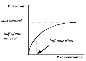
Figure 11‑3 - Removal as a Function of P Concentration
The mass of chemical precipitant formed is also calculated and added to the particulate inert inorganic component (xii). The stoichiometric amount of chemical sludge produced is based on the stoichiometry of the basic reaction. For example, in Equation 11.1, the mass of chemical precipitant (AlPO4) is 4.52 g per 1g of aluminum ion reacted.
The model provides the user with two dosage methods: mass flow based and flow proportional. The former requires the user to specify a continuous flow rate for the chemical, while the latter allows the user to specify a flow rate of chemical per unit flow of liquid entering the basin. The dosage rate can be set up as a manipulated variable to maintain the phosphorus at a specified set point at any location downstream of the chemical addition.
In addition to precipitating the phosphorus, the chemicals flocculate some of the colloidal organics into particulate matter. In the model this is simulated as a conversion of soluble inert COD and soluble substrate into particulate inerts and particulate substrate. The extent of flocculation will depend on the half-saturation constants for each species. These constants need calibration from plant to plant as the flocculation model is empirical.
Here is a detailed explanation of the constants of the Chemical Dosage menu item:
Number of chemicals: Currently four chemicals (alum, ferrous and ferric, plus a user defined) are available.
Dosage mode . Mass flow based: in mass/time units.
Flow proportional: in mass/volume units.
The following stoichiometry parameters (for all compounds) are found under the More… button, and are described in Table 11‑1.
Table 11‑1 - Chemeq Parameters
|
Parameter |
Description |
|
P precipitation stoichiometry |
gP/gMe precipitated stoichiometrically (if metal is in excess) |
|
soluble inert COD flocculation stoichiometry |
gCOD/gMe soluble inert COD converted to particulate inert COD (si to xi) |
|
soluble substrate flocculation stoichiometry |
gCOD/gMe soluble substrate converted to particulate substrate (ss to xs) |
|
metal hydroxide stoichiometry |
g of MeOH formed per g of metal added |
|
P precipitation half-saturation coefficient |
gP/m3 concentration at which half the Metal available for this reaction will be used to precipitate phosphorus |
|
soluble inert flocculation half-saturation coefficient |
gCOD/m3 concentration at which half the metal available for this reaction will be used to flocculate soluble inerts |
|
soluble substrate flocculation half-saturation coefficient |
gCOD/m3 concentration at which half the metal available for this reaction will be used to flocculate soluble substrate |
The stoichiometry for inorganic inert solids production from P precipitation that was available as a parameter in previous versions of this model (under the name chemdos) is now calculated from known stoichiometry.
In addition, the chemeq model is written as an equilibrium model, meaning that all precipitation and flocculation is assumed to happen instantaneously, and goes to completion within the flow-through of the In-line Chemical Dosage object.
All nitrogen and phosphorus fractions of COD components are recalculated for mass balance after the precipitation has taken place.
The chemeq model contains a P-removal dosage controller, which is available in the Input Parameters > Chemical Dosage menu (see Figure 11‑4).
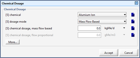
Figure 11‑4 – Dosage Controller Parameters
The controller allows users to specify a desired effluent P concentration, and back-calculates the required metal ion dosage, based on the stoichiometry settings.
The metaladd model is a semi-mechanistic model to assess the removal of soluble phosphorus due to metal addition. Following key assumptions are made in the model development.
1. The metal species exists in the form of Me(OH)3. All the other soluble and insoluble species of metal are not modeled. Thus, the model results outside the pH range of 6-8 may not be applicable.
2. Solubility product of the metal phosphates is used in estimating the amount of expected precipitates.
3. The solubility product is based on the PO43- ion which is estimated based on the solution pH and dissociation coefficient of H3PO4.
4. The removal mechanism is assumed to be instantaneous, therefore no volume of the reactor is considered.
Following mass balance equations may be written for different phosphorus components across the In-line Chemical Dosing object.
Mass Balance Equation for Me(OH)3 Concentration
Equation 11.2
![]()
Mass Balance Equation for Soluble Phosphorus Concentration
Equation 11.3
![]()
Mass Balance Equation for MePO4 Concentration
Equation 11.4
![]()
The equation describing the relationship among the metal ion, phosphate ion and the solubility product is as below:
Equation 11.5
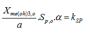
where:
Xme(oh)3,o = metal hydroxide concentration at outlet, gMe/m3
Xme(oh)3,in = metal hydroxide concentration at inlet, gMe /m3
Pme = metal dose, gMe /m3
a = stoichiometry conversion factor, gMe(OH)3 /g Me
Xmepo4,formed = concentration of formed precipitate, g MePO4/m3
b = stoichiometry conversion factor, gMe(OH)3/ g MePO4
c = stoichiometry conversion factor, g P/g MePO4
a = dissociation factor for estimating PO43- from total orthophosphate concentration
The set of above equations are solved simultaneously to calculate the soluble phosphorus removal in the in-line chemical dosing object. The main calibration parameter in the model is the solubility product of the metal phosphates. The default values are provided based on the evaluation of reported values in literature. The values however may need to be adjusted to account for the differences in wastewater characteristics, mixing regimes and other parameters which affect the P-precipitation process.
In addition to P-precipitation, the metaladd model also models the removal of colloidal COD (scol), soluble inert COD (si) and soluble organic nitrogen (snd) through flocculation. Following assumptions are used in the formulation of this empirical flocculation model.
1. The metal dose to flocculate unit soluble component is a function of the soluble component concentration.
2. The metal dose required per unit soluble component removed is expressed as an exponential function with minimum bound.
The equation for metal dose per unit ss removed can be expressed as below:
Equation 11.6
![]()
where:
F = metal consumed per unit soluble component at soluble component concentration C, g Me/g component
C = Concentration of soluble component, g/m3
Fmax = maximum metal consumption per unit soluble component, g Me/g component
Fmin = minimum metal consumption per unit soluble component, g Me/g component
ka = affinity factor, m3/g
The shape of the curve represented by the above equation is shown in Figure 11‑5:
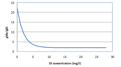
Figure 11‑5 – Curve Showing Relationship between the Soluble Components Concentration, and Require Metal Dose for Unit Soluble Component Removal
The integration of curve in Figure 11‑5 between the limits of Sin (concentration of soluble component in influent) and So (concentration of soluble component in effluent) results in the following expression. For a given metal dose and inlet concentration, the equation is solved to estimate the So, concentration of soluble component in effluent.
Equation 11.7
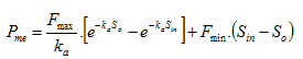
Equation 11.8
![]()
where:
Pme = metal dose, gMe/m3
Sin = concentration of soluble component in influent, g/m3
So = concentration of soluble component in effluent, g/m3
There are three parameters Fmax, Fmin and ka used in the model. The parameter Fmax may be interpreted as the amount of metal required to remove the said component at very low concentrations. It is general observation that the amount of metal required at lower concentration of soluble component is much higher than the metal amount required when the concentration of soluble component is higher. The parameter of Fmin, can be interpreted as the amount of metal required to remove the said component at high concentrations. The parameter of ka signifies the transition between the Fmin and Fmax. Higher values of ka will result in a very steep transition between the Fmin and Fmax, essentially improving the removal efficiencies. Conversely, lower values of ka will result in a mild transition and thus decreasing the removal efficiencies.
It is important to highlight here regarding the fate of the removed soluble components. As, the flocculation process does not cause any mass loss, the removed soluble compounds are just converted into their particulate state. The si, scol and snd are just transformed to xi, xs and xns states respectively.
It should be noted that the value of these parameters depends on the environmental conditions temperature, pH, mixing, and wastewater characteristics. Therefore, it is recommended that adequate calibration is performed to find the appropriate values for specific cases.
The model associated with this object is a simple empirical model where grit production is directly proportional to the flow coming in the grit chamber. The amount of grit produced (in grams per m3 of influent) is user specified.
The struvite precipitation reactor model represents an up-flow granular bed reactor with recycle. The model uses a bed fluidization model to estimate the granular bed height and the solid concentration in the effluent stream. An internal recycle is provided to achieve bed fluidization velocity required by the user. A typical layout showing the application of struvite reactor is as shown in Figure 11‑6. Some typical outputs from the struvite precipitation model are as shown in Figure 11‑7and Figure 11‑8.
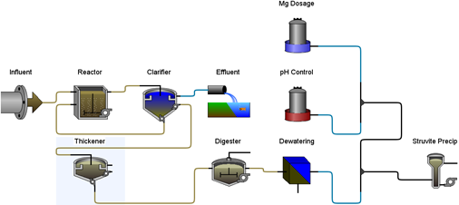
Figure 11‑6 - Typical Application of Struvite Recovery Reactor
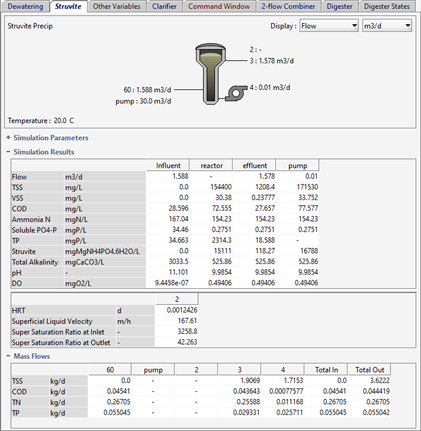
Figure 11‑7 - Typical Process Outputs for Struvite Reactor
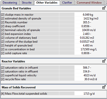
Figure 11‑8 - Typical Outputs for Solid Bed Volume and Expansion for Struvite Recovery Reactor
The empiric model associated with this object computes the fraction of surviving E. coli based on the detention time in the disinfection unit. The state variables are not affected by this model. The following equation is used as the model for computing the surviving fraction:
Equation 11.9
![]()
where:
survecoli = fraction of surviving E.coli
kill = rate of kill (m3/g/min)
ccl2 = chlorine dosage (g/m3)
tde = detention time (computed from volume/flow rate)
The chlorine dosage, rate of kill, and volumeof the unit are specified as operational parameters.
Chlorine is widely used for disinfection due to its cost effectiveness and high efficiency. In addition to its disinfection ability, chlorine can also reduce ammonia in the wastewater. However, a major concern of using chlorine as a disinfectant is the formation of toxic by-products such as Tri-Halo-Methane (THM) and Halo-Acetic Acid (HAA). The by-products formation can be extremely difficult to control and monitor due to hypochlorous acid’s high reactivity with various compounds present in wastewater. The optimization of chlorine dosages is often required to meet the disinfection requirement; to minimize the by-product formation and to meet the free chlorine discharge limits in the wastewater effluent to avoid damage to aquatic environment.
An empirical chlorination model is developed which can model the stoichiometric reactions between chlorine and ammonia to estimated combined and free chlorine residuals. The model also uses empirical relationships to estimate production THM, and HAA formation. Based on the available chlorine dosage, the disinfection effectiveness is also estimated.
The following expression is used to estimate instantaneous chlorine demand required by the organic compounds in water (Dharmarajah et al., 1991). The parameters of TOC and UV254 are used as representative organic compounds leading the instantaneous chlorine demand.
Equation 11.10
![]()
Where:
Cinst - instantaneous chlorine demand, mgCl2/L
![]() - empirical constant 1, -
- empirical constant 1, -
![]() - empirical constant 2, -
- empirical constant 2, -
![]() - empirical constant 3,-
- empirical constant 3,-
![]() - empirical constant 4,-
- empirical constant 4,-
sTOC - soluble total organic carbon, mg/L
![]() -absorbance at 254nm, cm-1
-absorbance at 254nm, cm-1
The UV254 is calculated by using a linear relationship between UV254 and the the soluble inert organics compounds (si) in wastewater.
A first order rate equation is used to model the decay of chlorine in wastewater.
Equation 11.11
![]()
Where:
Cavailable - available chlorine, mgCl2/L
Cdose - chlorine dose, mgCl2/L
kinact - decay constant, 1/hr
t - detention time (t10), hr
In the above expression, the chlorine dose is adjusted for any chlorine lost due to instantaneous demand. The net available chlorine is used in the chlorine-ammonia reaction and in by-product formation.
A typical breakpoint chlorination curve is as shown in Figure 11‑9. When chlorine is added to water containing ammonia, mono-chloramine is formed (zone 1). After all of the ammonia has reacted, the free chlorine reacts with the mono-chloramines to form di-chloramine and to nitrogen gas (zone II). The free chlorine residual starts to appear after breakpoint chlorination (zone 3).
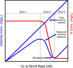
Figure 11‑9 - Breakpoint Chlorination [3]
Zone 1 occurs when the Cl2/NH3-N ratio is below 5.07 and involves the formation of chloroorganic and mono-chloramine compounds. The formation of di-chloramine and nitrogen tri-chloride is assumed to be negligible.
Zone 2 occurs when the Cl2/NH3-N ratio is above 5.07 and below 7.58. Chloramines and chloroorganic compounds are destroyed in this zone and the chloramines concentration becomes the lowest at breakpoint. In theory, breakpoint occurs when the Cl2/NH3-N ratio is 7.58, all the ammonia nitrogen is consumed by chlorine and free chlorine becomes available in zone 3. As the actual stoichiometric ratio may get affected by the water composition, the default stoichiometric ratio may be changed by the user in the model. The chlorination model was developed to reproduce the break point curve shown in Figure 11‑9. Using the above reaction scheme, the model calculates free chlorine (chlorine in HOCl and OCl- form), combined chlorine (chlorine in combined form with ammonia) and total chlorine (free + combined chlorine) in the system. Zone 3 is where the by-products formation is assumed to dominate as free chlorine concentration increases.
In zone 1, the ammonia gets converted chloroamine, hence no loss of nitrogen is considered. In zone 2 part of the chloroamine gets fully oxidized leading the nitrogen loss as nitrogen gas.
The formation of Trihalomethane (THM) occurs in the presence of hypochlorous acid (free chlorine). The expression used to determine the concentration of total trihalomethane (TTHM) formation is based on batch experimental work conducted by Amy et al. (1987) and is presented below.
Equation 11.12

Where:
CTTHM = total trihalomethane concentration (mmole/L)
UV254 = water UV absorbance at 254 nm; 1 cm path length (cm-1)
Cl2 = chlorine residual (mgCl2/L)
t = reaction time in the batch reactor (hr)
T = temperature (oC)
pH = pH after chlorine reaction (-)
Br = bromide concentration in raw water (mg/L)
The reaction time, t, is considered to be represented by the t50 value for a unit process. If chloramines are present, the TTHM formation has been observed to be reduced compared to when only chlorine is present. As a result, a factor of 0.2 times the general TTHM equation is applied when chloramines are present (USEPA, 1992).
Haloacetic Acid (HAA) formation is based on the AWWA Technical Advisory Workgroup’s (TAW) work. The data were obtained from a series of batch experiments, 96 hours in duration, using water from eight facilities. The work is presented in USEPA (1992), and is used as the default model. The expressions used to determine HAA formation are presented below and were obtained from the USEPA (1992).
Equation 11.13

Equation 11.14

Equation 11.15

Where:
CMCAA = monochloroacetic acid (ug/L)
CDCAA = dichloroacetic acid (ug/L)
CTCAA = trichloroacetic acid (ug/L)
sTOC = soluble TOC, mg/L
The Ai,j are the empirical model constants. It is assumed that the t50 value represents the reactor time t. If chloramines are present, a factor of 0.2 is applied to each of the individual HAA species concentrations, similar to the approach used for TTHMS when chloramines are present.
The following equation is used for estimating the log inactivation for disinfection.
Equation 11.16
![]()
Equation 11.17
![]()
Equation 11.18
![]()
Where:
t = time in batch reactor (min)
V
= volume of batch reactor (![]() )
)
Q
= flow rate of wastewater (![]() )
)
chlorine dose = chlorine present in the batch reactor (g/m3)
![]() ratio
=
baffling factor (short circuiting factor)
ratio
=
baffling factor (short circuiting factor)
pH = pH after chlorine reaction (-)
T = temperature (oC)
The werfuv model is based upon an empirical model presented in a 1995 WERF report comparing UV irradiation to chlorination (Water Environment Research Foundation, 1995). The model estimates the effluent coliform density:
Equation 11.19
![]()
where:
N = effluent coliform density (MPN/100mL)
n = empirical coefficient related to UV dose (unitless)
f = empirical water quality factor (unitless)
The empirical water quality factor, f, was determined from regression to be described by:
Equation 11.20
![]()
where:
SS = suspended solids concentration (mg/L)
UFT = unfiltered UV transmittance at 253.7nm (fraction)
A,a,b = empirical coefficients (unitless)
Four models are associated with this object: asce, empiric, simple and press. The models all simulate solids separation, but do so via different models that have been calibrated for different dewatering technologies.
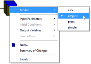
Figure 11‑10 - Dewatering Object Models
The asce model is based on a paper by the Task Committee on Belt Filter Presses for the American Society of Civil Engineers (ASCE, 1988). Based on this work, which involved information collected as part of a survey through the United States, a relationship was developed between the feed solids and cake concentration. The primary sludge fraction (i.e. percent of sludge for processing originating from primary sludge) is the main parameter in determining the cake solids from the unit. The solids capture is used to determine the centrate solids concentration and the developed relationship is used to determine the cake solids. A material balance is used to determine the two output flows.
The empiric dewatering model is used when modellers wish to specify an underflow solids concentration and flow rate, or specify a concentration removal efficiency along with either the underflow flow rate or solids concentration.
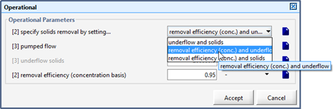
Figure 11‑11 - Operational Menu for Empiric Model
In the Operational Menu, users set the method for setting solids removal by selecting from the drop down menu. The relevant fields (pumped flow, underflow solids concentration, removal efficiency) are highlighted.
Once two of the three above options have been specified, the model performs a mass and flow balance (similar to the simple model below) to determine the flow and concentrations for the cake and filtrate streams.
In the simple model, the user inputs two operational parameters: Solids capture (%), and Polymer dosage (g/m3). From these two parameters, the dewatering parameters (under Parameters > Calibration) and the input solids concentration (Xi), the cake (Xs) and centrate (Xo) solids concentrations are calculated:
Equation 11.21
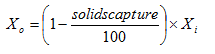
The optimal polymer
dosage and sludge treatability are used to define the performance
of the unit. The minimal sludge concentration for processing is a
limit concentration under which the unit will not operate. The cake
dry material content is a function of the treatability and the
expected content from easy to treat sludge at optimal polymer
dosage, hard to treat sludge at optimal, and no polymer
dosage.
Using the following mass balance, the output flow rates (Qo and Qs) can be computed:
Equation 11.22
![]()
The press model is based on the simple model but has, in addition, a parameter for the filter press surface area and a maximum load on the press. These two parameters are used to model the reduced efficiency of dewatering as the loading on the press increases.
The dewatering object should not be confused with the thickener object. The thickener is configured like a nonreactive settling tank. The Sedimentation Models are described in CHAPTER 8.
In certain solid-liquid separation devices (centrifuges, vortex separator etc.), the inorganic particulate matter may be removed at higher efficiency than the organic particulate matter due to difference in the density. Further, depending on the nature of aggregation/particle size of particulate matter, there may be differences in the relative removal efficiencies of different organic particulate matters.
In some of the sludge reduction systems (i.e. Cannibal Process), it is suggested that the inert organic material is preferentially removed by the solid-liquid separation device in the process. To model such processes, an empirical solid-liquid separation model (differential) is implemented in dewatering unit process considering differential removal of particulates depending on the characteristics of each particulate state variable.
In the differential settling model, the particulate matter concentration in the effluent is calculated based on the following equation:
Equation 11.23
![]()
where:
Xj,o = concentration of particulate state j in effluent, mg/L
Xj, in = concentration of particulate state j in influent, mg/L
aeff = removal efficiency
The concentration in the underflow (concentrated) stream is estimated by making a mass balance around the object.
Equation 11.24
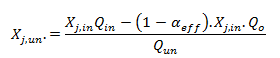
where:
Xj, un = concentration of particulate state j in underflow, mg/L
Qin = influent flow rate, m3/d
Qo = effluent flow rate, m3/d
Qun = underflow rate, m3/d
The underflow rate, Qun, is specified by the user as a constant value or as a fraction of the influent flow rate. The overflow rate is estimated by using the flow balance equation as below.
Equation 11.25
![]()
The soluble compounds in the influent are mapped to the effluent and underflow streams without any transformation.
The disc and belt microscreen objects also contain the empiric solids separation model, as described above, but with different default removal rates. The disc microscreen object is found in the “Tertiary Treatment” object group, and the belt microscreen object is found in the “Preliminary Treatment” object group. Both objects have only the empiric solids separation model.
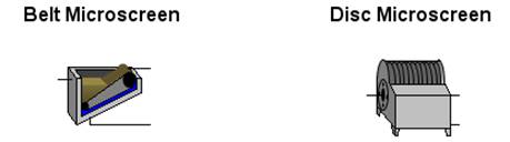
Figure 11‑12 – Belt and Disc Microscreen Objects
The hydrocyclone model found in the Biosolids Treatment section of the unit process table is a simple solids separation unit. It uses the same differential model as discussed above in the dewatering object. The solids capture rates for the various particulate components have been calibrated for typical performance. In particular, the solids capture rate for Anammox biomass is higher than that of the other biomass types, reflecting the heavier nature of the biomass which allows it to settle out preferentially.
The High-Rate unit process object is found in the “Biosolids Treatment” section of the unit process table. It contains the highrate solids separation model.
The highrate model is based on a vortex separator and retention treatment basin (RTB) model developed by Gall et al. (1997) and Schraa et al. (2004) for the high-rate treatment of wet weather flows such as combined sewer overflows (CSOs). The model has been applied to primary clarifiers, chemically enhanced primary clarifiers, RTBs, vortex separators, continuous backwash filters, and ballasted flocculation (e.g. Actiflo) and sludge recycle (e.g. Densadeg) systems.
The highrate model contains a hydraulic routing component and a settleability component. The hydraulic component of the model consists of algorithms to achieve dynamic volumetric and mass balances. The settleability component of the model includes a relationship between settleability and influent TSS concentration, and a relationship between settleability and the surface overflow rate (SOR). The settleability model for high-rate retention treatment basins is given below:
Equation 11.26
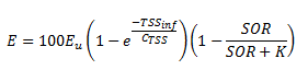
where:
E =concentration based removal efficiency (%)
Eu = ultimate settleable solids fraction (at high influent TSS)
CTSS = parameter that controls the exponential shape of the removal efficiency vs. Influent TSS relationship
TSSinf = influent total suspended solids concentration (mg/L)
SOR = surface overflow rate (m/h)
K = surface overflow rate a 0.5 Eu
In this model Eu, CTSS, and K are parameters that must be calibrated using measured data. Once calibrated, the model can be used to predict the removal efficiency achieved in a high-rate solids separation process, in terms of total suspended solids (TSS), given the influent TSS and the surface overflow rate (SOR).
The default settleability model parameters provided in GPS-X are based on data taken from studies conducted by the University of Windsor on a pilot-scale RTB operated at the Lou Romano Water Reclamation Plant (LRWRP) in Windsor, Ontario, Canada (Li et al., 2004) that used high doses of cationic polymer as the sole coagulant. A 3‑dimensional scatter plot of the pilot plant settleability data is given in Figure 11‑13. Tests that did not use polymer were removed from the data set. The circles represent data points and the lines or stems show where the points lie in the plane.
At a constant influent TSS, the removal efficiency was observed to decrease with increasing surface overflow rate. At a constant surface overflow rate, the removal efficiency increased exponentially with increasing influent TSS and leveled off at TSS values above approximately 500 mg/L.
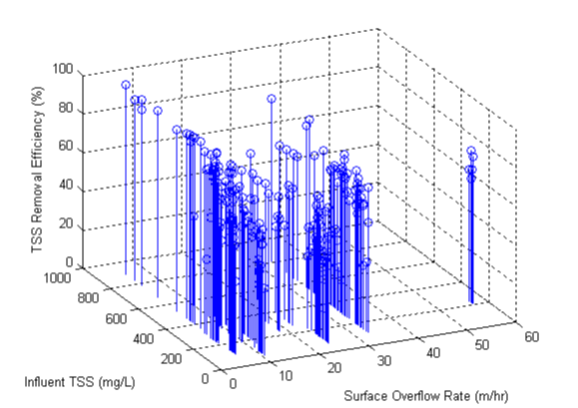
Figure 11‑13 - Plot of TSS Removal Effciency vs. Influent TSS and SOR (Pilot Data from U. of Windsor RTB)
The settleability model was calibrated to the entire set of pilot data shown in Figure 11‑13, using the optimizer tool in GPS-X and the sum of squares objective function (i.e. least squares parameter estimation). The calibrated parameter values are given below:
Eu = 0.86 (ultimate settleable solids fraction at high influent TSS)
CTSS = 82 mg/L (parameter that controls the exponential shape of the removal efficiency vs. influent TSS relationship)
K = 93 m/h (surface overflow rate at 0.5Eu)
A 3-dimensional plot of the calibrated settleability model is shown in Figure 11‑14. The model shows the same trends as the measured pilot data shown in Figure 11‑13. To check the performance of the calibrated settleability model, dynamic simulations were performed using the full RTB model and the measured influent TSS concentrations from the pilot tests. The simulation results showed reasonable agreement with the measured pilot study results given the estimated measurement error.
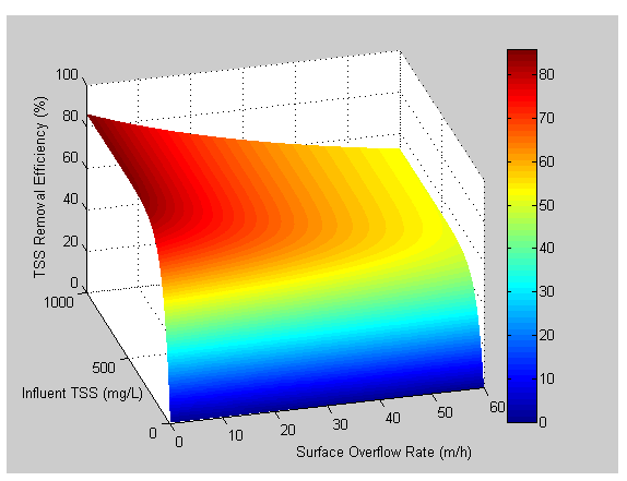
Figure 11‑14 - Plot of Calibrated Settleability Model
The Physical Setup form is accessed by right-clicking on the dewatering object and selecting Input Parameters > Physical. Figure 11‑15 shows the GPS-X form. The parameters are discussed below:
· Number of trains in operation: Specifies the number of high-rate treatment process trains.
· Surface area per train: Specifies the surface area of each train (assuming all trains have the same surface area). The default SI units are m2.
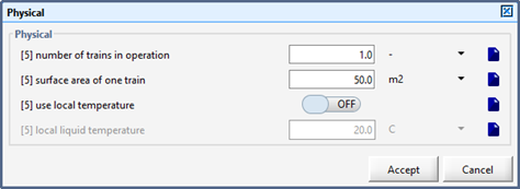
Figure 11‑15 - Operational Menu for High-Rate Treatment Model
The Operational Setup form is accessed by right-clicking on the dewatering object and selecting Input Parameters > Operational. Figure 11‑16 shows the GPS-X form. The parameters are discussed in the next section.
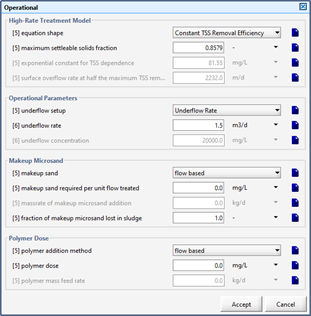
Figure 11‑16 – Operational Menu for High-Rate Treatment Model
Equation Shape – specifies the settleability model to be used. The user can select the following options: Constant TSS Removal Efficiency, Exponential Function of Influent TSS, Switching Function-Based SOR Relationship, Combined Equation
· Constant TSS Removal Efficiency: Uses the maximum settleable solids fraction to calculate the effluent TSS based on the influent TSS. For example, using E = 100Eu as the settleability model.
· Exponential Function of Influent TSS: Uses an exponential-based expression to calculate the effluent TSS based on the influent TSS. For example, using the following equation as the settleability model. This model increases TSS removal efficiency as the influent TSS increases
Equation 11.27
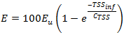
· Switching Function-Based SOR Relationship: Uses a switching function, based on the surface overflow rate (SOR) to calculate effluent TSS. For example, using the following equation as the settleability model. This model reduces the removal efficiency at higher SORs.
Equation 11.28
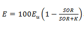
· Combined Equation: Uses the entire settleability equation to calculate the effluent TSS, based on the influent TSS and the SOR. For example, using Equation 11.26 (shown below) as the settleability model.
Equation 11.29
Maximum Settleable Solids Fraction: Specifies a maximum concentration-based TSS removal efficiency fraction. This is the highest TSS removal efficiency that can be achieved. The quantity is dimensionless (-) but can also be entered as a percentage
(%).Exponential constant for TSS dependence: This parameter controls the exponential shape of the removal efficiency vs. influent TSS relationship. Increasing this parameter will decrease the TSS-based removal efficiency. The default SI units are mg/L.
Surface overflow rate at half the maximum TSS removal efficiency: This parameter is the half-saturation coefficient in the removal efficiency vs. SOR switching function-based relationship. Increasing this parameter will increase the TSS removal efficiency. The default SI units are in m/d.
Underflow Setup: This drop-down menu allows the user to select how the underflow rate and concentration are calculated. (Underflow Rate, Underflow Concentration)
· Underflow Rate: The underflow rate is specified and GPS-X calculates the underflow concentration using a mass balance.
· Underflow Concentration: The underflow TSS concentration is specified and GPS-X calculates the underflow using a mass balance.
Underflow Rate: This is the underflow rate used when the Underflow Rate option is selected. The default SI units are m3/d.
Underflow Concentration: This is the underflow TSS concentration used when the Underflow Concentration option is selected. The default SI units are mg/L.
The Outputs menu is accessed by right-clicking on the dewatering object and selecting Output Variables. Figure 11‑17 shows the Output Variables menu options.
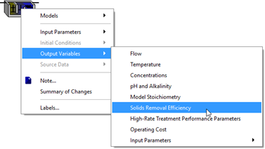
Figure 11‑17 - Output Variables Menu in High-Rate Treatment Model
The Output Variables menu options that are unique to the high-rate treatment model are discussed below:
Solids Removal Efficiency: The solids removal efficiency form is shown in Figure 11‑18. The user can plot or track the solids removal efficiency.
High-Rate Treatment Performance Parameters: The high-rate treatment process loading rates form is shown in Figure 11‑19. The user can display the surface overflow rate and/or the solids loading rate.
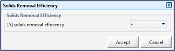
Figure 11‑18 - Solids Removal Efficiency Output Variable Form
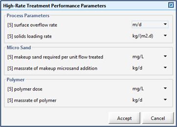
Figure 11‑19 - High-Rate Treatment Performance Parameters Output Variables Form
The advanced oxidation unit process is found in the Tertiary Treatment panel in the unit process table. The model is an empirical model for modeling soluble COD removal from wastewater using oxidising agents like ozone, hydrogen peroxide etc.. The user specified oxidant dose and oxidant effectiveness factor are used to oxidize soluble organic compounds like soluble inert COD, colloidal COD, readily biodegradable COD, acetic acid COD, propionic acid COD and methanol COD. The nitrogen and phosphorus fractions associated with the soluble inert COD are hydrolysed, thus increasing the concentration of ortho-phosphorus and ammonia-N concentration.
The input for maximum COD removal efficiency is used to control the residual COD in effluent at chemical overdose. The influent flow and chemical dose are used to estimate the mass of chemical required for treatment.
The Black Box object contains three models: Empiric, Pipe, and Interchange
The empiric model contains a number of empirical equations that can be set up to change the value of the BOD, TKN and the suspended solids between the input connection point and the output connection point.
The available regression equations are:
1) constant
2) proportional
3) linear
4) quadratic
5) exponential
6) power
7) user-defined
After choosing the correlation type, the user specifies what variable is the independent variable (either influent flow, influent concentration or both). Finally, the user must supply the parameters in the regression equation. Equation 11.30 and Equation 11.31 are typical regression equations that can be set up using the Black Box object.
One independent variables (solids), with proportional regression
Equation 11.30
![]()
Two independent variables (flow and concentration), with linear regression
Equation 11.31
![]()
There are two options available to specify the state variable mapping: From menu, and From custom macro:
From custom macro: State variable mapping is specified in the custom macro file in the interchange model file (accessible by clicking on the interchange option from the model menu). More advanced mapping calculations can be performed in the custom macro (see Figure 11‑20). For details on how to write custom calculations, see the Customizing GPS-X chapter in the User’s Guide.
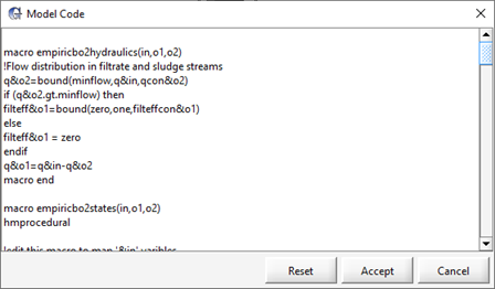
Figure 11‑20 – Custom Interchange Macro
The pipe model can be used to simulate the lag effect caused by significant residence times in pipes or channels between unit process objects. By default, GPS-X does not simulate any travel time between objects.
The pipe model is a plug-flow tank model without any biological reactions.
The energy consumed in a pumping system depends on the pumped flow rate, pump head and pump efficiency. For a give pumped flow rate, the energy consumption will depend on pump head and pump efficiency. The required pump head for a pumping system has comprises of static head and dynamic head loss in the pipes, valves and fittings. While static head is independent of the pumped flow rate, the dynamic pump head is a function of pumped flow rate and piping system. The pump efficiency is also a function of the pump flow rate and normally available from the pump characteristic curve. The simple pump energy models applied to variable flow conditions typically use a constant head and constant efficiency, leading to inaccurate estimation of pumping requirement. These models are also not suitable to compare energy performance of pumps having different pump characteristics curves. Therefore, in situations where large variation in the pumped flow rates are expected, better energy consumption estimates can be made giving adequate attention to pump characteristics curve.
The advanced pump energy model in GPS-X allows user to dynamically estimate the pump head and pump efficiency under variable pump flow conditions using the pump characteristics curves. Two pump models are implemented 1) Fixed speed pump model and 2) Variable speed pump model.
System Curve Characteristics
The pump model requires that a system curve is defined for the pumping system. In the GPS-X model following equation is used to define the system curve.
Equation 11.32
![]()
Equation 11.33
![]()
Where:
![]() = static system head, m
= static system head, m
![]() =
static dynamic head, m
=
static dynamic head, m
![]() =
dynamic head-loss coefficient, -
=
dynamic head-loss coefficient, -
![]() = flow rate in the system, -
= flow rate in the system, -
The model requires an input value for hstatic, the static head of the system. In addition to this, a point (Q, hdynamic) on the dynamic head curve needs to be specified by the user. This point on the curve is estimate the dynamic head-loss coefficient (K). The GPS-X input screen for system curve characteristics is as shown below in Figure 11‑21 and Error! Reference source not found.:
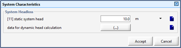
Figure 11‑21 - Inputs for System Curve Definition – Static Head
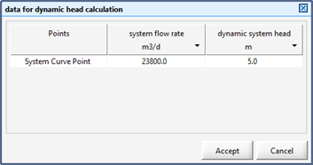
Figure 11‑22 - Inputs for System Curve Definition - Dynamic Head
The pump model requires an input of pump characteristics curve. The user can provide the pump characteristics curve for a specific speed of the pump by setting pump flow rate, pump head and pump efficiency for a selected number of points on the pump curve. An example is shown in the table below:
Table 11‑2 - Sample Pump Characteristics
|
Points on Pump Curve |
Pump Flowrate |
Pump Head |
Pump Efficiency |
|
( - ) |
(m3/hr) |
(m) |
(%) |
|
Point 1 |
0 |
22.7 |
0.0 |
|
Point 2 |
250 |
21.8 |
19.1 |
|
Point 3 |
500 |
20.7 |
20.0 |
|
Point 4 |
750 |
19.8 |
37.3 |
|
Point 5 |
1000 |
18.7 |
63.6 |
|
Point 6 |
1250 |
17.6 |
72.7 |
|
Point 7 |
1500 |
16.5 |
78.2 |
|
Point 8 |
1750 |
15.6 |
82.7 |
|
Point 9 |
2000 |
14.5 |
84.5 |
|
Point 10 |
2250 |
13.6 |
86.4 |
|
Point 11 |
2500 |
12.4 |
86.4 |
|
Point 12 |
2750 |
11.3 |
85.5 |
|
Point 13 |
3000 |
10.0 |
82.7 |
|
Point 14 |
3250 |
8.5 |
77.3 |
|
Point 15 |
3500 |
6.9 |
69.1 |
For any given flow rate, the model uses pump characteristics curve and system head loss properties to calculate the system operating point (Figure 11‑23). Based on the pump operating point, the model calculate pump efficiency, number of pump and energy consumption in pumping.
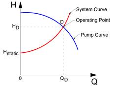
Figure 11‑23 - Pump operating point based on pump and system curves
In this model, user can run the pump in a variable speed mode and estimate the energy saving that may be achieved by converting a fixed speed pump to a variable speed pump for a given system conditions. An ON and OFF switch is provided in model for the variable speed pump. In addition to above user inputs required for the fixed speed pump, additional inputs for the minimum and maximum speed of the pump are required. The variable speed model is built with an energy optimization algorithm in which the model finds a pump speed at which consumption of pumping energy is minimized. The typical outputs for the variable speed pumps are:
1) Number of pumps required to be operated
2) speed of the pumps
3) efficiency of the pump
4) system head, pump head
The following affinity equations are used to calculate the flow rate, pump head and power requirement at different speed of the pump.
Affinity Law #1: ![]()
Affinity Law #2: ![]()
Affinity Law #3: ![]()
where,
Q1 = flow rate at N1 speed, m3/d
Q2 = flow rate at N2 speed, m3/d
H1 = pump head at N1 speed, m
H2 = pump head at N2 speed, m
P1 = power absorbed at N1 speed, kW
P2 = power absorbed at N1 speed, kW
The change in the pump curve at different pump speeds are as shown in Figure 11‑24.
.
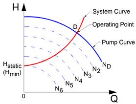
Figure 11‑24 - Pump curves at different pump speeds
In the variable speed pumping, a VFD power efficiency factor is introduced to take into account the power. The equation for calculating different power consumptions are as shown below.
Phydraulic = ρ·g·Q·H
Pshaft = Phydraulic / ηpump
Pmotor = Pshaft / ηmotor
Pinput = Pmotor / ηVFD
where,
P = power, kW
ρ = water density, kg/m3
g = gravity acceleration, m/s2
Q = flow rate, m3/d
H = total head, m
ηpump = pump hydraulic efficiency, -
ηmotor = motor efficiency, -
ηVFD = VFD (variable frequency drive) efficiency, -
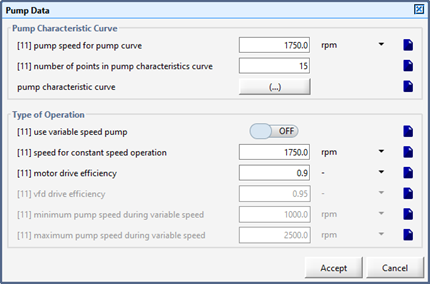
Figure 11‑25 - Pump Characteristics Curve - Pump Speed for Pump Curve
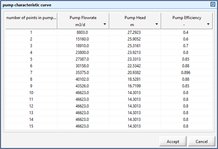
Figure 11‑26 - Pump Characteristic Curve Inputs
Based on the input data of system head loss, pump characteristics and a given flow rate, the model find the operating point for the pump. It estimates the number of pumps required to pump the flow and efficiency of the pump at the operating point.
A typical output for a pump system pumping a diurnal flow is shown in Figure 11‑27.
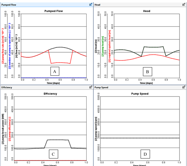
Figure 11‑27 - Typical Output from a Fixed Pump Speed
It can be seen that when the pump flow rate increases to more than the pumping capacity of a single pump, two pumps become operational, each pumping half of the total flow rate [Figure 11‑27 A]. At this point since the flow rate are decreased for each pump, the change in the pump operating point leads to reduced pump efficiency [Figure 11‑27 C]. This reduced pump efficiency increases the energy consumption significantly for the pumping system. During the model calculation, head used in the energy calculation is the greater of the system head and pump head Figure 11‑27 C]. In general, the pump head should always be higher than the system head for proper pumping. This condition should always be checked by the user. If the pump head is lower than the system head, an alternative pump having more appropriate pump characteristics curve should be used. In this particular example, constant speed is used throughout the simulation.
The typical outputs from the variable speed pump model are as shown in Figure 11‑28. Following observations may be made by comparing the outputs of variable speed pump and fixed speed pump.
1) The pump head follows the required system head more closely [Figure 11‑28 B] than that in the fixed speed pump system. Synchronization of the pump head with the system head results in reducing energy consumption.
2) The increase in the speed of the pump follows the increase in the flow rate. The optimum speed of the pump is estimated to achieve the lowest power consumption.
3) The pump efficiency for the variable speed system 0.84 – 0.88 as against the efficiency variation in the range of 0.77 – 0.88 for the fixed speed system.
4) The power consumption for the variable speed pump varies from 62-132 kW while for fixed speed system the observed range was 100-180 kW.
It is clear from the above analysis that the variable speed pumps can offer significant energy saving in a pumping system where flow variations are large.
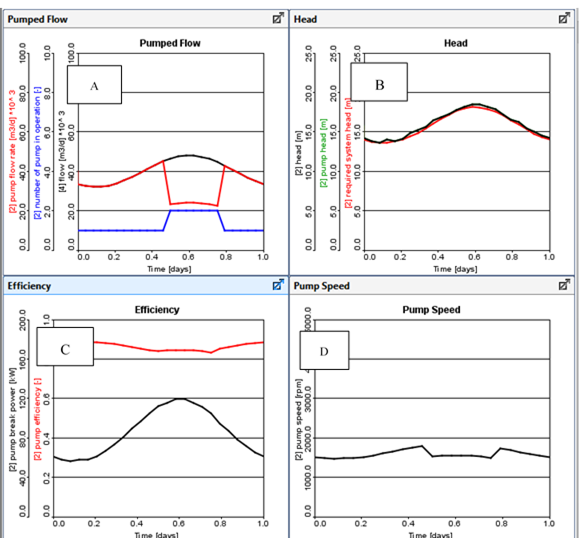
Figure 11‑28 - Typical Outputs for Variable Speed Pump

The building object does not have any effect on the treatment of liquid or solids streams. It is used for the estimation of energy requirements of buildings on the treatment plant site. Users can place as many building objects as needed on the GPS-X layout. The building object calculates the energy usage for HVAC, lighting, refrigeration, and miscellaneous in the building. Based on the energy usage, the operational cost for the building is calculated.
Heating, cooling, and HVAC energy requirement for the building is estimated using conductive heat transfer equation as shown below:
![]()
where:
![]() = heat
transferred per second (
= heat
transferred per second (![]() )
)
![]() = area (
= area (![]() )
)
![]() =
temperature difference
=
temperature difference![]() )
)
![]() = thermal resistance parameter (
= thermal resistance parameter (![]() )
)
![]() = performance factor (-)
= performance factor (-)
HAVAC energy can be estimated in GPS-X by specifying temperatures, physical and heat resistance parameters of the wall, HAVAC efficiency as stated by the manufacturer,
Lighting
Light energy usage for the building is calculated by specifying the quantity and wattage of the lighting device.
Refrigeration
Refrigeration energy usage is estimated based on conductive heat transfer through the walls, frequency of usage (air changed in the cooler), and refrigerated material load. In GPS-X, the user specifies the temperature, physical and heat resistance parameters of the cooler, cooler performance as stated by the manufacturer, refrigerated load characteristics, and usage frequency.
Other Miscellaneous
Other miscellaneous energy required for the building can be specified under this section. The input can be specified by entering a power value or entering a fraction of the total building power usage.
Energy requirements and cost estimations for the building are shown in the Operating Cost output menu, as shown in Figure 11‑29 below. Note that the energy requirement for the building is included in the miscellaneous category for the plant-wide energy demand and operating cost calculations.
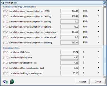
Figure 11‑29 – Operating Cost Output Menu
Effluent Quality Index model in effluent unit process uses the user specified concentration limits and compound specific weight factors to estimate 1) time duration for which a plant is under violation with respect to specified concentration limits 2) estimates the instantaneous and moving average Effluent Quality Index and 3) estimate the net and moving average Effluent Quality index.
The WQI is representative of the effluent pollution load to a receiving water body and is estimated using the expression provided in COST simulation benchmark (EC, 2002).
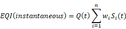
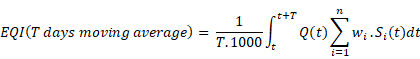
Where:
![]() – Instantaneous effluent flow rate, m3/d
– Instantaneous effluent flow rate, m3/d
n – number of compounds in EQI estimation (-)
![]() – weight factor of compound
in EQI (-)
– weight factor of compound
in EQI (-)
![]() –instantaneous concentration of compound in
EQI estimation
–instantaneous concentration of compound in
EQI estimation
T – time period for moving average calculation
The net WQI, which is defined as the weighted pollution load over and above the violation concentrations, is also calculated in the model as below.
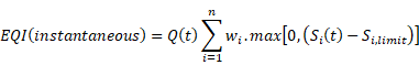

Where,
![]() – violation concentration of compound in EQI
estimation
– violation concentration of compound in EQI
estimation
By default, a total of 9 compounds including TSS, COD, BOD, NH3-N, TKN, TN, NOx-N, Ortho-Phosphorus, and total phosphorus are used in the EQI calculation. User can exclude contribution from any of these compounds by setting the weight factor of that compound to zero.
The cumulative time of violation for a specific parameter is estimated by the integrating the time during which the plant is out of compliance with respect to that parameter.
The cumulative time of violation is divided by the total time to estimate the time fraction in violation.
This chapter discusses the models found in the Tools and Process Control objects. The toolbox object is found in the Tools section of the unit process table. The Process Control section of the unit process table contains several objects. Each model is described in separate sections below.
![]()

The sampler model is found in the toolbox object, and will sample any stream either at regular time intervals (i.e., take a sample every `x' hours) or in proportion to the flow rate of that stream (take a sample every `x' m3 of flow). It reports either daily or total simulation run average values.
The sampling tool parameters are accessed by selecting Parameters > Set up in the Process Data menu. These parameters are detailed below:
Label of sample stream: This is the label of the stream being sampled. All of the state and composite variables in this stream are sampled.
Sampling mode ( Off / Flow Proportional / Regular Time Intervals ): This switch controls how the stream is sampled. The stream can be sampled in proportion to the flow or at regular time intervals.
Sampling period ( Daily / Total Run ): This is the time period used when calculating the averages of the sampled values. The averages can be calculated on a daily basis or for the entire run.
Take a sample every (m3): This parameter controls how often the stream is sampled when the sampling mode is set to Flow Proportional.
Take a sample every (hour): This parameter controls how often the stream is sampled when the sampling mode is set to Regular Time Intervals.
![]()
The ph tool is found in the Toolbox object in some libraries, and allows the user to estimate the pH of a wastewater stream in the layout, or do pH estimation directly from parameters entered into the menu. These two options are available in the pH Model Set up menu (Figure 12‑1).
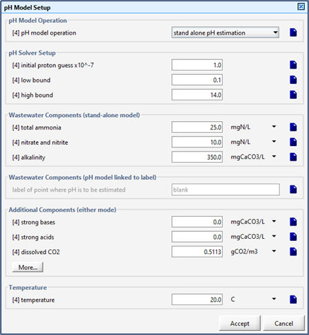
Figure 12‑1 - pH Model Set up Menu
The pH model operation menu item specifies whether the calculation is a standalone pH estimation using the components under the Wastewater Components (stand-alone model) header, or uses the components from a specific flow point in the plant layout.
If you select link pH estimation to label, the calculation will use the concentrations of ammonia, nitrate, etc., from the stream label specified in label of point where pH is to be estimated. If you would like to estimate the pH at several different points throughout the plant, place one Toolbox object per pH calculation into the layout, and link each box to a different point in the layout where pH is to be estimated.
The calculation is based on a model developed by Vavilin et al. (1995). The model is simplified to include only strong bases, strong acids, total ammonia, total acetate, and total carbon dioxide. The model uses an iterative process, in combination with the concentration of each component, to determine the pH value.
The relationship between the concentration of a component and the concentration of its ions is related through a dissociation constant (K). The concentration of hydrogen ion is used to determine pH:
Equation 12.1
![]()
The initial pH identified on the pH solver set up control form is used to calculate the initial concentration of hydrogen ion. An example of this control form is shown in Figure 12‑1. The default initial guess for pH is 7.
A second control form, shown in Figure 12‑2, is used to input various equilibrium and temperature constants.
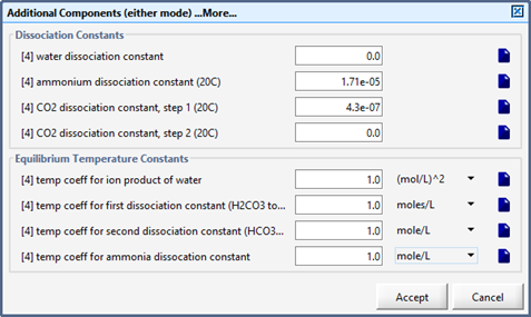
Figure 12‑2 – Component Control Form
These concentrations are used in a series of five equilibrium equations that form the basis for the pH model:
Equation 12.2
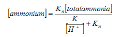
Equation 12.3
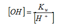
Equation 12.4
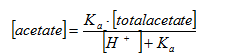
Equation 12.5
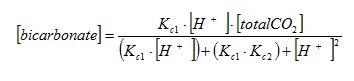
Equation 12.6
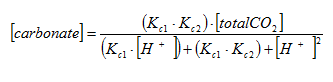
where:
Kn = ammonium dissociation constant (mol/L)
Ka = acetate dissociation constant (mol/L)
Kw = water dissociation constant (mol/L)
Kc1 = CO2 dissociation constant – step 1 (mol/L)
Kc2 CO2 dissociation constant – step 2 (mol/L)
The dissociation constants used in these equations can also be input on the control form shown in Figure 12‑2. The default dissociation constants are taken from the literature. The ammonium dissociation constant is corrected for temperature.
To properly reflect the presence/absence of added alkalinity (lime addition, etc.) the alkalinity state variable salk is assumed to be all carbonate alkalinity that is available (and completely dissociated) for acid neutralization.
In the above equations, totalCO2 is the total CO2 available (converted to equivalent charge). Because the alkalinity is assumed to be in the form of completely dissociated CaCO3, a 2+ charge cation is also assumed present in the equilibrium system.
The above equations are combined with the charge balance shown below:
Equation 12.7
![]()
An implicit nonlinear equation solver is used to solve this system of equations for [H+]. The calculated pH values are bounded by the low bound and high bound parameters shown in Figure 12‑1.
Once the solution is complete and the concentrations of the ionized components have been calculated, the concentrations of the non-ionized components are calculated from the speciation equation shown above.
The calculated pH and the concentrations of the individual components can be displayed on an output form similar to that shown in Figure 12‑3. This pH model is also used in the HPO (High Purity Oxygen) object for pH estimation.
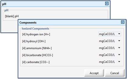
Figure 12‑3 – Sample pH Outputs
The lowpass model is found in the toolbox object, and can be used for analog or digital filtering, or a combination of both. The input signal is fed to a first-order analog filter, a first-order digital filter, and a zero-order sample-and-hold. Any of these components may be used or bypassed. This is done by setting the filter type as Analog, Digital, or Analog+Digital, and by setting sample and hold to either ON or OFF. When the filter type is set to OFF, both filters are bypassed and the final output is either the input signal or the sampled input signal, depending on the state of the sample and hold setting. A signal flow diagram is shown in Figure 12‑4. In this figure, the switches are set for a digital filter with sampling.
First-order linear filters have one tuning parameter, the cutoff frequency ωc, which corresponds to the corner frequency, i.e. the reciprocal of the filter time constant. The amplitude ratio of a first-order system at the corner frequency is 1/√2, with corresponding phase lag φ=45 degrees’
With u(t) and y(t) representing the input and output of a first-order filter respectively, the filter models are:
Analog:
Equation 12.8
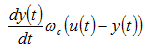
Digital:
Equation 12.9
![]()
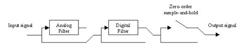
Figure 12‑4 – Signal Flow Diagram for the lowpass Model
One menu of parameters is defined for the lowpass model. It is accessed from the Tools Process Data menu by selecting Parameters > Filter Settings. The available parameters are detailed below:
Input signal: The cryptic name of the variable to be filtered.
Filter type (Analog / Digital / Analog+Digital / Off): The value of this parameter determines whether the signal flows through the analog or the digital filter, or both.
Analog filter cutoff frequency: The corner frequency of the first-order analog filter, or the reciprocal of its time constant.
Digital filter time step: The value of the time interval used in the digital filter model. It is also used as the sampling time when Sample and hold is set to ON.
Digital filter cutoff frequency: The corner frequency of the first-order digital filter, or the reciprocal of its time constant.
Sample and hold (ON - OFF): The value of this parameter determines if the digital filter output is sampled and held for the sampling period specified above.
Digital filtering without sampling is useful if the filtered signal is to be used in a unit that already implements a sample-and-hold on its input.

The ON/OFF controller object is found in the Process Control panel. On/off controllers are simple forms of feedback control. This type of controller is used in a wide variety of common applications. For example, household heating and cooling systems operate using on/off control.
The ON/OFF controller parameters are divided into two groups: control variable parameters, and manipulated variable parameters. The control variable parameters are accessed by selecting Parameters > Control Variable from the Tools Process Data menu. The manipulated variable parameters are accessed by selecting Parameters > Manipulated Variable from the Tools Process Data menu.
Controller (ON – OFF): A value of ON indicates that the controller is active; a value of OFFindicates that the controller is not active (i.e., not adjusting the manipulated variable). This should not be confused with the `on' and `off' states of the on/off controller.
Controller sampling time: This parameter determines the length of time between controller executions. A high value (corresponding to a long interval between executions) may be appropriate for slower processes (e.g., MLSS control using the sludge wastage rate), while other processes may require faster sampling frequencies.
Control variable (CV) with label: The cryptic name of the variable to be controlled.
Upper bound: The upper bound on the controlled variable. If the value of the controlled variable exceeds this value, then the value of the manipulated variable will be set to its low setting.
Lower bound: The lower bound on the controlled variable. If the value of the controlled variable is less than this value, then the value of the manipulated variable will be set to its high setting.
Manipulated variable (MV) with label: The cryptic name of the manipulated variable.
MV setting when CV is at low limit: The value of the manipulated variable is set to this value when the value of the controlled variable is less than its lower bound.
MV setting when CV is at high limit: The value of the manipulated variable is set to this value when the value of the controlled variable exceeds its upper bound.
MV initial value: The value to assign to the manipulated variable until the controlled variable crosses either its upper or lower bound.

The PID object contains two models: PID, and PIDforward. Regular PID controllers are widely used in industrial applications because of their simplicity and good performance. PID is an acronym for Proportional, Integral, Derivative, which are the three modes of the PID controller. In continuous form, the PID controller algorithm is given by:
With derivative kick protection OFF:
Equation 12.10
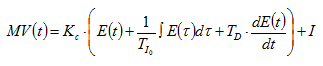
With derivative kick protection ON:
Equation 12.11
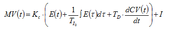
where:
MV = manipulated variable
E = error (setpoint-controlled variable)
Kc = proportional gain, a controller tuning constant
TI = integral time, a controller tuning constant
TD = derivative time, a controller tuning constant
I = initialization constant
The individual modes of the PID controller can be used individually or in pairs; common combinations include P-only and PI control, in addition to full PID control. The output of the PI controller, for example, includes the first two terms in the PID controller expression above; the output of any combination can be calculated similarly. The proportional mode is given by:
Equation 12.12
![]()
The integral mode is given by:
Equation 12.13
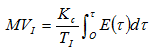
The derivative mode is given by:
Derivative kick protection OFF
Equation 12.14

Derivative kick protection ON
Equation 12.15
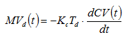
Since the vast majority of PID controllers are now implemented using digital computers, the discrete form of the PID algorithm is used more frequently than its continuous form. Accordingly, all controllers in GPS-X are modelled in discrete form. Bounds on the manipulated variable are frequently used to reflect limitations due to physical equipment or safety. Therefore, the PID algorithms implemented in GPS-X have the following forms, where Dt represents the controller execution interval.
With derivative kick protection OFF:
Equation 12.16
![]()
With derivative kick protection ON:
Equation 12.17
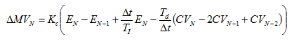
Equation 12.18
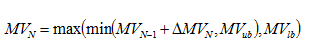
With derivative kick protection OFF:
Equation 12.19
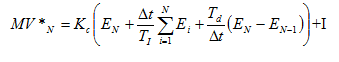
With derivative kick protection ON
Equation 12.20
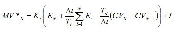
Equation 12.21
![]()
The velocity form is obtained by differencing the position form of the PID controller. When using the velocity form, one calculates the change in the value of the manipulated variable that is to be implemented, as opposed to the absolute value calculated by the position form of the algorithm. The velocity form has certain advantages over the position form; in particular, it is naturally protected against reset or integral windup. This condition occurs when a persistent, nonzero setpoint error results in a large value of the integral mode of the PID, forcing the control action to `saturate' (i.e. to maintain the manipulated variable at its minimum or maximum value). Even when the setpoint error returns to zero, the control action remains saturated when the position form of the PID algorithm is used. When using the velocity form, the control action can return within the control range after one sampling period.
Derivative kick protection is a commonly used modification to the standard PID algorithm. The modification, which affects the derivative mode only, prevents large `jumps' from occurring in the manipulated variable as the result of setpoint changes. These jumps occur because a discrete setpoint change introduces a discontinuity into the error signal, resulting in an "infinite" derivative (in the continuous case), or a large value in the difference error signal (in the discrete case). Therefore, it is recommended that derivative kick protection be used for all PID controllers, unless the behaviour described above is specifically desired.
Derivative filtering is another strategy by which large jumps in the manipulated variable can be prevented. Filtering reduces the effect of sudden setpoint changes and high frequency noise present in the error signal, which may produce large values of the error derivative. When derivative filtering is selected, the signal fed to the derivative mode of the PID (error or controlled variable) is passed through a discrete first-order filter before being used in the calculation of the derivative mode. The filter is tuned by a single parameter, the cutoff frequency, which corresponds to the filter's `corner frequency'. (i.e.‑the reciprocal of its time constant)
The parameters available for PID controllers are listed below. These parameters are divided into two groups: control variable parameters, and manipulated variable parameters. The control variable parameters are accessed by selecting Parameters > Control Variable from the Tools Process Data menu. The manipulated variable parameters are accessed by selecting Parameters > Manipulated Variable from the Tools Process Data menu.
In addition to the PID controller in the tools object, PID controllers for common variable pairings are built into many of GPS-X's process objects. For example, a PID controller for controlling the dissolved oxygen concentration is available in the plug flow tank object. These controllers have essentially the same parameters as the PID controller in the tools object except that the manipulated variable and possibly the controlled variable have already been defined.
Controller (ON - OFF): This parameter determines whether or not the PID controller is active.
Setpoint for control variable: This is the value of the setpoint for the controlled variable. The controller acts to keep the controlled variable at the setpoint.
The following parameters are accessed by clicking on the More... button in the Control Variable form. Only the parameters in the Controller Set up sub-section are discussed here. For a discussion on the Controller Tuning sub-section see Tuning PID Controllers.
Controller form (Full Position / Velocity): This parameter is used to specify which form of the PID controller equation is used (position or velocity). The default velocity form is recommended because it has built-in protection against integral windup.
Controller type (P / PI / PID): This parameter specifies the modes to be used in the PID controller. Using the PI option is recommended in most cases. When using the P option, the offset between the controlled variable and the setpoint cannot be completely eliminated.
Control variable with label: This is the cryptic variable name for the controlled variable including the appended stream label.
Controller sampling time: This is the length of time between controller executions. If this parameter is too large the control performance will be poor and possibly unstable.
Proportional gain: This is the controller tuning constant, Kc.
Integral time: This is the controller tuning constant, TI.
Derivative time: This is the controller tuning constant, TD.
Controller effect on controlled var - direct (ON - OFF): Since the value of the proportional gain in GPS-X must be positive, this parameter controls the `direction' of the controller. If a positive step in the manipulated variable results in a positive change in the controlled variable (at steady-state), i.e. the process gain is positive, then this parameter should be ON(e.g. an increase in air flow causes an increase in DO). Otherwise, it should be OFF(e.g. an increase in wastage rate causes a decrease in MLSS concentration).
Derivative kick protection (ON - OFF): When this setting is ON the manipulated variable is prevented from making large jumps in response to setpoint changes. This parameter is only applicable when the controller type is set to PID.
Derivative filtering (ON - OFF): The derivative filter is used to filter the signal fed to the derivative mode of the PID controller.
Cutoff frequency: This is the derivative filter's corner frequency (i.e. reciprocal of its time constant).
Manipulated variable w/o label: This is the manipulated variable name without the stream label.
Label of manipulated variable: This is the stream label of the manipulated variable.
Value of manipulated variable: This is the initial value of the manipulated variable.
Minimum value: This is the lower bound on the manipulated variable.
Maximum value: This is the upper bound on the manipulated variable.
Many different techniques exist for tuning PID controllers. While an in-depth discussion of these techniques is beyond the scope of this manual, some general guidelines are provided below.
A simple and conservative approach to controller tuning is as follows:
· Start with a small proportional gain and a large integral time; set the derivative time to zero (0). As a rough rule of thumb:
o Use a value of 0.5/Kp as a starting value for the proportional gain (Kp is the steady-state process gain, defined as the change in the controlled variable at steady-state for a one-unit change in the manipulated variable).
o Use a value of 1.5t as a starting point for the integral time (t is the time constant of the first-order response that most closely approximates the controlled variable response to a step in the manipulated variable).
· Gradually increase the proportional gain until further increases result in deterioration in control performance.
· Gradually decrease the integral time until further decreases result in deterioration in control performance.
· Gradually increase the derivative time.
· Fine-tune the parameters as needed.
A facility for tuning PID controllers based on the Ciancone correlations for setpoint changes is available for all PID controllers in GPS-X. The PID tuning parameters calculated using the Ciancone correlations are based on estimates of the process gain, dead time, and time constant, obtained by a least-squares fit of the time series data collected under tuning mode.
The controller tuning parameters for the PID controller are accessed by selecting Parameters > Control Variable > More... in the Process Data menu of the tools object. Setting tuning to ON starts the tuning mode. The controller sampling time must be set to an appropriate value. The process should have been brought to steady-state, or reasonably close to steady-state, prior to the activation of the tuning mode. This may be done with or without a PID controller currently ON. While this mode is active, a step input is applied to the manipulated variable, forcing the controlled variable to be perturbed.
This mode may be deactivated by manually setting Tuning to OFF, at which point suggested PID tuning parameters will be displayed in the simulation Log window, based on an analysis of the time series data collected during the tuning operation. It is not necessary to wait for a new steady-state before turning off the tuning operation, but it may be desirable to do so. Tuning parameters will also be suggested if the simulation terminates while the tuning mode is ON.
The estimates of the process parameters (i.e. process gain, dead time, and time constant) may be tagged for display in the Output Variables menu of the object or stream associated with the controller.
The other settings which affect the operation of the tuning mode are:
Fractional step size: The size of the step to be applied in the manipulated variable, specified as a fraction of its initial value.
Time of step: The interval of time that will elapse between the activation of the tuning mode and the application of a step in the manipulated variable.
Maximum possible dead time: Upper bound on admissible values of dead time in the first-order plus dead time model. This may be used to reduce the time required to compute tuning constants, or may be used to force a dead time of zero in the model used to derive the tuning constants.
While operating in tuning mode, time series data of the manipulated and controlled variables are sampled (at each controller sampling time) and stored in arrays of fixed maximum size. Data for 3000 sampling times can be stored. If that capacity is to be exceeded, a warning will be displayed, and a scrolling time window that will retain data for the last 3000 sampling times will be initialized. This should not be a limitation in most cases, as this storage capacity is enough for data sampled every 10 minutes over 20 days. The storage capacity is a global setting labeled controller tuning array size, found in General Data > System > Parameters > miscellaneous. If this value is increased, the layout must be recompiled for the change to take effect, i.e., this value may not be changed inside a scenario. For more information on tuning PID controllers, consult Marlin (1995) or Perry and Chilton (1973). The Ciancone correlations are presented and discussed in Marlin (1995).

Users can select the PIDforward model in this PID controller object, by right-clicking on the object and selecting Models > pidforward. With a feedforward controller, an input disturbance is measured and the controller adjusts the manipulated variable to compensate for the disturbance before the controlled variable deviates from its setpoint. Feedforward control is usually combined with feedback control to retain the beneficial properties of feedback.
The pidforward model of the Tools object combines a PID controller for feedback and a lead/lag algorithm for feedforward control. Lead/lag feedforward control is a simple feedforward strategy that provides enough flexibility for most applications. The PID controller algorithm is presented in the section entitled PID Controllers above. In this section we present the lead/lag algorithm.
A feedforward term may be added to the feedback control action of the PID controller when measurement of a process disturbance is available. The lead/lag feedforward controller is represented in transfer function form as:
Equation 12.22
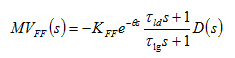
Its time-domain representation is given by:
Equation 12.23
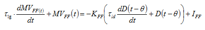
where:
MVFF = additional control action provided by feedforward control
KFF = the feedforward gain, a controller tuning parameter
q = the feedforward dead time, a controller tuning parameter
tld = the feedforward lead time, a controller tuning parameter
tlg = the feedforward lag time, a controller tuning parameter
IFF = the initialization constant of the feedforward controller
When both the process and disturbance dynamics are represented by first-order plus dead time models, perfect feedforward control can in principle be achieved if one:
· Sets the feedforward gain KFF to the disturbance-to-process gain ratio;
· The dead time q to the difference between disturbance and process dead times (possible only when the process dead time is less than the disturbance dead time);
· tld the lead time to the process time constant; and,
· The lag time tlg to the disturbance time constant.
The feedback control action is calculated from a PID control algorithm as described above, and the feedforward control action is added to it as follows:
Feedforward/Feedback (PID in velocity form):
Equation 12.24
![]()
Feedforward/Feedback (PID in position form):
Equation 12.25
![]()
where:
ΔMVNFF = the change in feedforward control action obtained from discretizing the lead/lag algorithm and the superscript FF refers to the feedback controller.
The parameters of the pidforward model are presented in three menus: Manipulated Variable, Controlled Variable, and Disturbance Variable. Feedback control parameters are located in the Controlled Variable menu and feedforward control parameters in the Disturbance Variable menu.
The feedforward controller parameters found in the Disturbance Variable form are detailed as:
Feedforward controller (ON- OFF): The feedforward component of the controller is activated by this switch.
Disturbance variable with label: The cryptic name of the disturbance variable including the stream label.
Controller sampling time: The length of time between controller executions.
Feedforward gain: The feedforward controller tuning parameter, KFF.
Leadtime: The feedforward controller tuning parameter, tld.
Lag time: The feedforward controller tuning parameter, tlg. The ratio of lead to lag times should usually be kept below 2:1 to minimize the effects of noise.
Dead time: The feedforward controller tuning parameter, q.
Negative feedforward gain (ON - OFF): This parameter controls the `direction' of the controller. The `normal' sign of the feedforward gain is negative. This occurs when both the process and disturbance gains have the same sign, in which case this setting should be ON (the default value). Otherwise, it should be OFF.
For information on tuning Feedforward/Feedback controllers, consult Marlin (1995).

The timer is used to schedule and control intermittent plant operations. For example the timer control can be used to implement intermittent aeration in an activated sludge tank. Another application is the desludging of a primary settler.
The timer works in cycles. At the start of each cycle the timer sets its manipulated variable to a pre-defined ‘on’ value. The manipulated variable is kept at this value for a user-defined fraction of the cycle. For the remainder of the cycle, the manipulated variable is set to a pre-defined ‘off’ value. This is ideally suited for intermittent aeration because the controller can turn on the air flow at regular intervals for a user defined length of time.
The timer control parameters are accessed by selecting Parameters > Set up in the Process Data menu. These parameters are detailed below:
Controller (ON - OFF): This switch activates the timer.
Manipulated variable with label: The cryptic name of the manipulated variable including the appended stream label.
Cycletime: The length of one cycle.
Ontime in one cycle: The length of time (starting at the beginning of the cycle) that manipulated variable value is set to the `on' value during a cycle.
Value of manipulated variable when on: The `on' value of manipulated variable.
Value of manipulated variable when off: The `off' value of manipulated variable.

The multivar model is used in conjunction with the Advanced Control Module. See the Advanced Control Module Manual for details on using multivariable controllers in GPS‑X.

The Flow Timer Model is a modification of the regular Timer model GPS-X. The Flow Timer Model is developed to address the specific needs to define daily intermittent flows using average daily flow rates. The main difference between the timer and flow timer model is in the choice of input variable. In the timer model, the input values of the variables are instantaneous values while in the Flow Timer Model, the flow variables are the average value in the cycle.
The input form for the Flow Timer Model is as shown in Figure 12‑5.
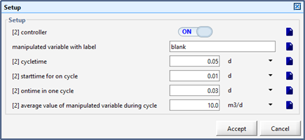
Figure 12‑5 - Flow Timer Menu
Controller – The controller switch is used to turn the flow timer model ON/OFF. Flow will be controlled, only when the controller is switched ON.
Manipulated variable with label – This input variable is used to specify the cryptic variable name of the flow variable that needs to be controlled.
Cycletime – This input variable is used to specify the total duration of the cycle including the ON and OFF time.
Start time for ON cycle – This input variable controls the start time of the cycle.
Ontime in one cycle – This input variable defines the duration of ON cycle.
Average value of manipulated variable during cycle – This input variable defines the average flow rate during the whole cycle.
The default setup of the flow controller defines a cycle of total length of 0.05d; the cycle remains OFF for 0.01d, gets ON at 0.01d and remains ON until 0.04d. The flow is OFF from 0.4d-0.5d. This cycle then repeats itself.

Some of the operations at wastewater treatment plant follow a repeating schedule. For example, the sludge wasting schedule may require wasting on the weekdays and no wastage on weekends. Until now, these repeating schedules were modeled by inputting the scheduled inputs through a file input. This approach requires preparation of file inputs for the duration of dynamic simulation. To simplify modelling a repeating schedule, a new scheduler model is implemented in the toolbox object of the GPS-X. The structure of the scheduler model is generic and can be used to model cyclic schedules of operation in a treatment plant. The scheduler model can control flow rates, split ration and any other model input variable.
The scheduler model can be selected by right-clicking on the tool box object and selecting scheduler. The scheduler model is useful when the treatment plant is operated in a well-defined cycle containing many different phases and in each phase a set of model variables is manipulated in a well-defined manner. In the current scheduler model, a set of 15 model variables can be manipulated to define complex operational schedules in treatment plants.
The Scheduler model requires the following information:
1. Number of phases in a cycle
2. Time duration of each phase
3. Cryptic names of model variables which are manipulated in a cycle
4. Value of each model variable in each phase of the cycle
The input data to the model is set by using the input form of the scheduler model. The input data form is as shown in Figure 12‑6. A brief explanation of each input variable is given below.
Number of phase in sequence: This variable defines the number of distinctive phases in a cyclic-sequence. The default value is set to 8.
Duration of each phase: This variable defines the time duration of each phase. The sum of the time duration of each phase is equal to the total sequence (cycle) time. Figure 12‑7 shows the input form for setting the duration of each phase.
Cycle start phase: This defines the phase at which the cycle starts. The value of the variable can be between 1 to number of phases defined above.
Cryptic name of model variables– This defines the cryptic names of the model variables which are manipulated in each phase. By default, a maximum of 10 model variables can be used to set the sequence. All the variables are set to blank (nothing is manipulated in the sequence). To include a model variable in the scheduler set-up, the blank should be replaced by the full cryptic name of the variable available in the layout. For example, to set the influent flow rate for an influent object in the sequence, the blank variable can be replaced by qconinf (qcon is the cryptic for influent flow rate and inf is the stream id). If there are more than one variable, they can be similarly defined.
TIP: To see the cryptic name of a variable, you may point the cursor over the variable description name in the data input window. The cryptic variable name is displayed for few seconds in a small window.
Value of model variable in each phase: The value of a model variable during each phase can be set here. For example, to set the values of control variable in each phase, click on the (…) button to the right of the control variable to open the input value form for model variables.
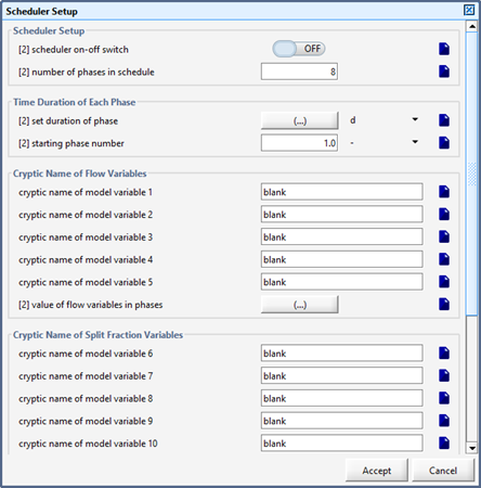
Figure 12‑6 - Input Form for the Scheduler Model
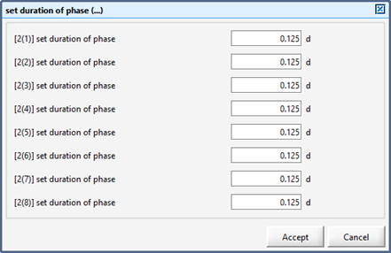
Figure 12‑7 - Input Form for Setting Duration of Each Phase
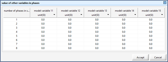
Figure 12‑8 - Input Form for Setting the Value of Control Variable in Each Phase of a Sequence
GPS-X contains operating cost models for most of the objects in the process table. Each object can be set up to calculate costs for energy, chemical dosage and sludge handling (as appropriate to that object).
This chapter discusses the structure of the operating cost models, and their use and calibration.
For each of the wastewater unit process objects in GPS-X, a set of operating costs has been assigned. These costs reflect the typical operating costs associated with that particular unit process.
GPS-X can be used to dynamically simulate these operating costs in the same way that it dynamically simulates the wastewater unit process itself.
The different types of operating costs modelled are:
· Aeration energy cost
· Pumping energy cost
· Mixing energy cost
· Heating energy cost
· Other miscellaneous energy cost
· Chemical dosage cost
· Sludge handling cost
The following sections described each cost in detail.
An aeration energy cost can be calculated for unit processes that have aeration, such as the CSTR, plug flow tanks, SBR, etc. The amount of energy required to supply the calculated level of aeration depends on several factors, including blower/compressor efficiency, headloss, etc., and the factors included in the oxygen transfer model (See Modelling of Oxygen Transfer in Chapter 6).
GPS-X can simulate two different aeration methods - mechanical and diffused air. If mechanical aeration is chosen, an aeration power (kW) is entered. If diffused aeration is chosen, the power requirement is calculated as shown in Equation 6.27 and Equation 6.28 in Chapter 6.
The wire power is multiplied by the energy price ($/kWh), and then integrated over time to determine the total cost for aeration energy during the simulation
Energy required for the pumping of water and wastewater is modelled in GPS-X using the following equation:
Equation 13.1
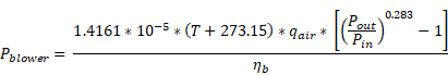
![]()
![]()
Where:
![]() = Blower power, kW
= Blower power, kW
![]() = Air temperature, ºC
= Air temperature, ºC
![]() = Air Flow rate, m3/d
= Air Flow rate, m3/d
![]() = Air pressure at discharge, kPa
= Air pressure at discharge, kPa
![]() = Air pressure at the inlet, kPa
= Air pressure at the inlet, kPa
![]() = Blower efficiency, -
= Blower efficiency, -
![]() = Atmospheric pressure, kPa
= Atmospheric pressure, kPa
![]() =
inlet pressure loss, kPa
=
inlet pressure loss, kPa
![]() = diffuser submergence, m
= diffuser submergence, m
![]() = head loss in piping and diffuser, kPa
= head loss in piping and diffuser, kPa
The energy value is multiplied by the energy price ($/kWh), and integrated over time to determine the total cost for aeration energy during the simulation.
For blower energy costs, the head value represents the sum of the actual head and the piping headloss. There is no additional equipment headloss as with aeration energy costs.
The mixing energy cost model describes the use of energy for mechanical mixing operations.
Ssers are required to input the required mixing power usage per unit volume (kW/m3). This value is multiplied by the volume of the tank, and then multiplied by the energy price ($/kWh) and integrated over time to determine the total cost for the simulation.
The heating energy cost model describes the use of energy for heating individual unit process operations such as digesters, or activated sludge units in cold environments.
Users are required to input a heating power usage per unit volume (kW/m3). This value is multiplied by the energy price ($/kWh) and integrated over time to determine the total cost for the simulation.
The miscellaneous energy cost model describes the use of energy for various mechanical operations such as gates, arms, rakes, moving bridges, etc.
Due to the complex nature of estimating these types of energy requirements, users are required to input a flat rate of energy usage (kW). This value is multiplied by the energy price ($/kWh) and integrated over time to determine the total cost for the simulation.
Some unit process objects in GPS-X allow for chemical addition as part of treatment (some influents, equalization tank, DAF, dewatering units, etc.).
In each case, the total chemical dosage cost is:
Equation 13.2
![]()
where:
chemicalcostperday = chemical dosage cost ($/d)
chemprice = chemical price ($/kg)
chemdosagerate = hydraulic head (kg/d)
This daily cost is integrated over time to determine a total cost for the simulation.
Several objects in GPS-X have connection points which represent thickened or dewatered sludge (e.g. dewatering unit). A sludge disposal cost can be associated with these flows to determine a sludge handling cost.
The cost is determined by multiplying the per-unit disposal cost by the rate of sludge disposal:
Equation 13.3
![]()
where:
disposalcostperday = sludge disposal cost ($/d)
disposalcost = disposal price ($/m3)
sludgerate = sludge disposal rate (m3/d)
This daily cost is integrated over time to determine a total sludge disposal cost for the simulation.
Operating cost parameters are found in two places:
General Data Forms: Right-click on an open spot in the layout. These forms contain general operating cost parameters that apply to the entire layout (i.e., energy prices and schedules).
Operating Cost Parameter Forms (in each object): These forms contain operating cost parameters that are specific to each object (i.e., headloss, pump efficiency, chemical cost).
Operating cost
variables controlling the price of energy can be found in the
Layouts > General Data > System > Input Parameters
> Operating Cost Settings menu (See Figure
13‑1).
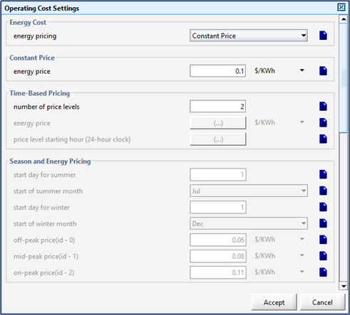
Figure 13‑1 – General Operating Cost Parameters Form
The price of energy can be set in two different ways, by selecting from the Energy Pricing menu:
· Time-based Pricing (energy price varies throughout the day)
· Seasonal Pricing
When Constant Price is selected, the energy price is set to the value entered on the form. This value can be changed in a scenario or by placing the price on an interactive controller, or set constant for the entire simulation.
When Time-based Pricing is selected, the energy price will cycle through a user-defined set of prices on a user-defined schedule. The number of different energy prices is unlimited. This mode can be used to simulate lower energy costs during the night.
The Seasonal Energy Pricing model allows the user to evaluate the cost of power consumption under a dynamic price structure based on season, weekday, weekend and hour of the day. The model is an extension of the Time-Based Pricing model which only allows specification of daily variation in energy price. The start day and month for each season is required to be set by the user.
In seasonal pricing model, two seasons of summer and winter are set each of which can have different energy pricing structure. Three tiers of off-peak, mid-peak and on-peak prices can be specified by the user.
In each season, weekdays and weekends are allowed to have any hourly price structure using the three tiers of pricing level.
The input form for the seasonal price model is as shown below.
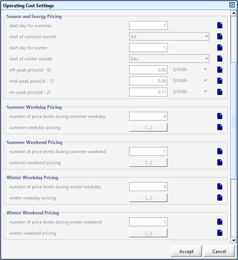
Figure 13‑2 – Input menu for seasonal price model
In seasonal price model, date and time set in the Simulation Setup menu is used to determine the season and day name. This information is used to determine the energy price based on the user inputs.
For all objects, the operating cost model parameters can be found in the Parameters > Operating Cost menu, and its associated More... button. The values entered on these forms are specific to each object. These objects can be tagged and placed on controllers, etc., as with any other parameter.
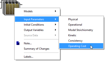
Figure 13‑3 - Operating Cost Menu
The operating cost model parameters shown in the Operating Cost parameters form depend on the object and choice of model.
Similar to the operating cost parameters, the associated output variables are divided into general and object-specific groups.
Operating cost output variables can be selected from the Layout > General Data > System > Output Variables > Operating Cost menu. These output variables include the energy price; total energy, chemical and sludge disposal costs for the entire layout; and the total operational cost for the layout (sum of the total energy, chemical and sludge disposal costs).
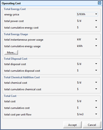
Figure 13‑4 - Layout Operating Cost Display Form (total for all objects)
For all objects, operating cost model output variables can be selected from the Output Variables > Operating Cost menu by right clicking on the effluent connection point.
The output variables available include energy usage and sludge disposal rates as well as total energy, chemical and disposal costs for that particular object. The specific costs calculated (and available in this menu) depend on the operating costs associated with the particular object and model.
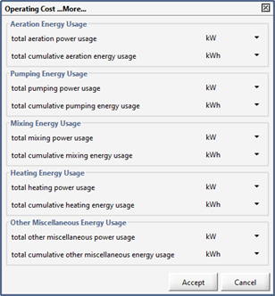
Figure 13‑5 - Object-Specific Operating Cost Display Form
The operating cost models in GPS-X are designed to simulate typical operating costs found in typical wastewater treatment facilities. The models are populated with parameters that give costs for typical plants.
To calibrate the models to the behavior of the plant being simulated, the user will need to adjust various parameters in the models. This list can be useful in guiding calibration.
Enter the hydraulic head and headloss for the system, if known. Otherwise, use the defaults. Calibrate with the blower efficiency and diffuser headloss.
Enter the hydraulic head and headloss for the system, if known. Otherwise, use the defaults. Calibrate with the pump efficiency and/or piping headloss
As these calculations are a flat “flow multiplied by price” calculation, the model is calibrated by adjusting the price parameter (flow is calculated or set elsewhere).
As these calculations are done on a “per unit volume” basis, make sure that you have the correct volume for the unit. Adjust the power per unit volume usage as needed.
The miscellaneous energy uses are flat rates, so they are calibrated by adjusting the rates as appropriate.
This chapter describes the GPS-X optimizer and its associated forms. More detail on the maximum likelihood objective function and the statistical tests provided in the solution report can be found in Appendix A and Appendix B, and the Optimizer Solution Report. The complete list of nomenclature used is found in Appendix C: Nomenclature. The references cited in this chapter are listed in Appendix D: References.
The optimizer is a module designed to minimize the value of a user-selected objective function by adjusting the free variables in this function. In the case of parameter estimation, these free variables are the unknown process parameters. The optimizer uses the Nelder-Mead simplex method (Press et al., 1986) for minimization. The algorithm has been modified to handle bounds on the optimization (i.e. free) variables.
The simplex method is a multi-dimensional procedure that does not rely on gradient information. The algorithm searches through the multidimensional "surface" using a direct search method to find a local minimum of the objective function.
The procedure starts with an initial point in the multi-dimensional parameter space and then generates new points in space by perturbing the initial point a scaled amount along each parameter direction. This leads to p + 1 points in space that define a polyhedron (the simplex) where p is the number of optimization variables. The points are called the vertices of the simplex.
At each iteration, the simplex method reflects the vertex with the highest function value (worst point) through the centroid of the remaining p points of the polyhedron. The amount of reflection is controlled by a reflection constant. If the reflected vertex is the new best point (lowest function value) then the polyhedron is expanded along the direction of reflection. The amount of expansion is controlled by an expansion constant. If the expanded vertex is better than the reflected vertex it is taken as the new best point.
If after the reflection step the reflected vertex is worse than the second worst vertex on the previous iteration, the polyhedron is contracted. The reflected vertex is contracted through the centroid of the remaining p vertices if it is the new worst point. If the reflected vertex is the new second worst point, the worst point is contracted through the centroid. The amount of contraction is controlled by a contraction constant.
When a contraction step is unsuccessful, the polyhedron is shrunk by moving the vertices toward the best point. The amount of shrinkage is controlled by a shrink constant.
At each step checks are made to ensure that the parameter bounds have not been violated. If they have been, the new vertex is moved back inside the bounds.
When the optimizer termination criteria are satisfied, the optimizer runs one additional simulation using the parameter values from the best point found during the iteration process. There is the possibility of encountering a local minimum that is not the global minimum of the objective function. This is a problem that is common to most optimization algorithms. As a result, it is important to solve optimization problems (e.g. parameter estimation or process optimization problems) from a number of different starting guesses to ensure that the optimizer has found the global minimum.
If the user requests the printing of confidence limits or derivative information (See Summary of the Optimizer Settings and Parameters section below) the optimizer conducts additional simulations to generate numerical derivatives.
The constants that control the reflection, expansion, contraction,
and shrinkage of the polyhedron in the simplex method can be
accessed by selecting
Layout > General Data > System > Input Parameters
> Simulation Tool Settings and then clicking on the
More... button in the Optimizer sub-section. The
resulting form is shown in Figure 14‑1. You can
change any of the constant values if you wish. The parameter
entitled scaled step size in initial guess is used to
control the initial perturbation size.
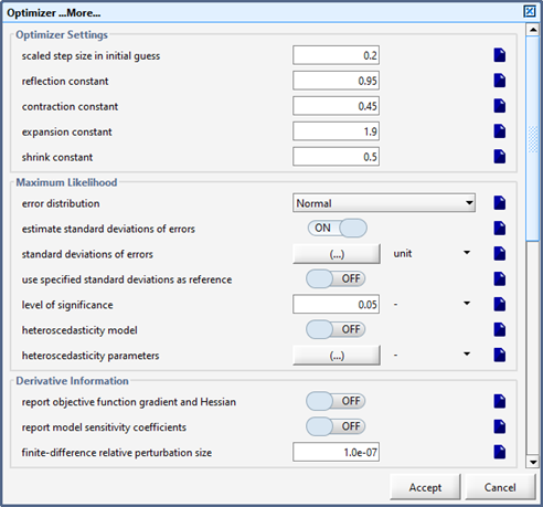
Figure 14‑1 – Form Containing the Simplex Method Constants
The list of objective functions available in GPS-X is given below:
Absolute Difference
Equation 14.1
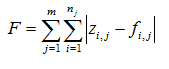
Relative Difference
Equation 14.2
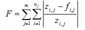
Sum of Squares
Equation 14.3
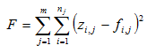
Relative Sum of Squares
Equation 14.4
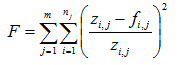
Maximum Likelihood
Equation 14.5
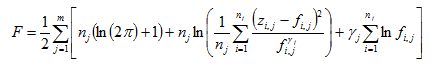
In the objective function expressions given above the following nomenclature is used:
zi,j = the measured value of response j in experiment i.
fi,j = the value of response variable j predicted by the process model in experiment i
gj = the heteroscedasticity parameter for response j
m = the number of measured response variables
nj = the number of experiments (i.e. observations) for response j
These objective function types are accessed by clicking on the inverted triangle beside the Optimize icon and then selecting Type from the drop-down menu.
In general, the maximum likelihood objective function should be used when doing parameter estimation. This objective function calculates statistically optimal parameter estimates based on assumptions on the nature of the measurement errors. The sum of squares objective function is a special case of the maximum likelihood objective function derived using further simplifying assumptions and can also be used. It is equivalent to the maximum likelihood objective function when there is only one response or target variable. Further details on parameter estimation and the maximum likelihood and sum of squares objective functions can be found in Appendix A of this chapter.
The other objective functions can be used for curve fitting when calculating statistically optimal parameter estimates is not a concern.
In addition to data fitting applications, GPS-X can be used for process optimization. For example, GPS-X can calculate the operating conditions for your process model that optimize some measure of process performance, such as operating cost or effluent quality.
To solve this type of problem in GPS-X you need to treat the problem as a data fitting exercise. For example, if you want to minimize the value of a certain model variable you need to specify an arbitrarily small target value for the model variable in a .dat file and have the optimizer minimize the difference between the calculated variable value and the target value using the absolute difference objective function. This is equivalent to minimizing the model variable directly. The target value should be made small enough so that the optimizer cannot reach it.
You are not limited to using one performance measure. You can select a number of different performance measures and have GPS-X optimize these variables simultaneously by fitting them to user-supplied targets.
There are four different criteria used to terminate the optimizer:
1. Parameter Tolerance: The maximum size along a parameter dimension is defined as the difference between the largest value of this parameter from among all of the simplex vertices, and the smallest value of this parameter from among all of the simplex vertices. This maximum size is scaled by dividing it by the difference between the upper and lower bounds for this parameter. If the maximum sizes for all of the parameter dimensions are less than the parameter tolerance, the optimization process is terminated.
2. Objective function tolerance: If the range (largest minus smallest) of objective function values covered by the simplex vertices is less than the objective function tolerance, the optimization process is terminated. Meeting this criterion without satisfying criterion 1 may indicate that the objective function is not very sensitive to some parameters.
3. Scaled termination value for objective function: If the objective function value at the current best point in the simplex is less than the user-specified final objective function value, the optimization process is terminated. This final value should be positive and small in magnitude. This criterion is not used with the maximum likelihood objective function. It is only applicable for the other objective functions because their values have a lower bound of zero (a perfect fit).
4. Maximum number of optimizer iterations: The optimization process is terminated if the maximum number of iterations is reached.
Satisfaction of any one of these four criteria will result in termination of the iterative optimization process. These criteria provide a trade-off between the length of the optimization run and the proximity to an optimal solution.
The specific values used for the termination criteria can be accessed from the General Data menu. Right-click in an empty region of the drawing board to display the menu and select System > Input Parameters > Simulation Tool Settings to display the form shown in Figure 14‑2.
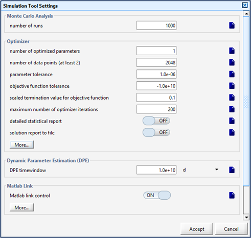
Figure 14‑2 – Optimizer Form Containing the Termination Criteria Settings
A termination criterion can be disabled by specifying a large negative value for it. The objective function tolerance is disabled by default.
The optimizer module is equipped to handle three different types of process measurements: time series measurements, long term operational data that are averages of the original process measurements, and on-line measurements. Each type of measurement set leads to a different type of optimization problem in GPS-X. These optimization types can be accessed by clicking on the inverted triangle to the right of the Optimize and selecting Type.
This optimization type is the one normally used for both parameter estimation and process optimization in GPS-X. It is designed to handle both time series and steady-state measurements.
For this type of optimization, you enter your measured data into a text file with a .dat extension. This text file should follow the naming and formatting conventions discussed in the GPS-X User's Guide.
For parameter estimation involving a dynamic model, the data entered into the text file will be a set of time series values for each of the response variables. In GPS-X the response variables are referred to as target variables.
Steady-state optimization is a time series-type optimization with only one data point for each target variable. The steady-state solver is used and the simulation has a stop time of 0.0. This type of optimization is useful for calibrating the model to data reported as daily, weekly or monthly averages. Data of this type are typically obtained from composite samples and thus do not accurately reflect the time dynamics of the real process. In a steady-state optimization, the average data are used as the targets and selected model parameters are adjusted to fit these targets.
When doing process optimization, you enter single target values for your process performance measures at the desired points in time. As mentioned earlier, you should also make sure to use the absolute difference objective function.
GPS-X will fit your model to the measured data using the objective function that you select. If you prepare output graphs to display the predicted values of the model, GPS-X will automatically display the measured values provided in the .dat file on the graphs.
GPS-X will draw a new curve for the predicted values at each optimization iteration, in order to track the progress of the optimizer. At the end of the optimization process, final predicted responses are displayed so that you can visually assess the fit. An example of this type of graph is shown in Figure 14‑3.
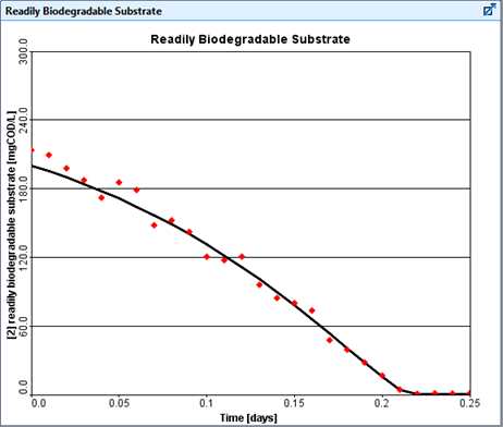
Figure 14‑3 - Example GPS-X Output Graph Showing Measured Data (+ Markers) and the Predicted Response (Continuous Line)
GPS-X also has a sophisticated dynamic parameter estimation procedure (DPE). DPE is designed for the estimation of time-varying parameters. It can be used with on-line data or on a set of off-line time series data. For details on using on-line data, see the Advanced Control Module Manual.
The motivation behind DPE is that parameters in process models are often not constant, but vary with time. For example, the oxygen mass transfer coefficient in an aerated tank is often slowly time-varying.
Dynamic parameter estimation is also useful for estimating parameters in poorly understood processes. In these cases, the model structure is likely to be incorrect. As a result, the model may only be able to represent the data well over short time intervals. In this case, using DPE will help compensate for the model error and allow acceptable fitting of the measured data.
Another situation in which dynamic parameter estimation is useful is when you are interested in detecting process changes and upsets. If for example a model parameter is found to be relatively constant during normal process operation but is sensitive to process changes, you can track this parameter using the DPE feature and on-line data to help provide an early warning of process changes or disturbances.
In GPS-X, dynamic parameter estimation is done by applying the time series optimization approach mentioned earlier to a moving time window. Instead of estimating parameters from an entire set of data, GPS-X calculates a set of parameter estimates for each time window using the parameter estimates from the previous time window as a starting guess. This approach can be used on a data file that is continually updated with new blocks of data or on a static file of time series data. You can use any of the objective functions that are available for time series optimization when doing dynamic parameter estimation.
The length of the time window controls how often the parameters are updated. The shorter the time window, the more often the parameters are updated. When using short time windows, it may be necessary to filter the data to eliminate noise so GPS-X does not fit the noise.
To ensure proper termination of the optimization routine when using the DPE feature, it is suggested that the time window and the communication interval be chosen such that the time window is an integer multiple of the communication interval.
This section
discusses the optimizer form that is accessed by selecting
General Data > System > Input Parameters >
Simulation Tool Settings > Optimizer > More…. The
upper portion of this form is shown in Figure 14‑2.
The lower portion of the form is shown below in Figure
14‑4.
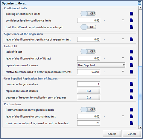
Figure 14‑4 - Bottom of Optimizer Form
The termination criteria found on this form were discussed under Termination Criteria in this chapter. The form accessed from the More... button in the Optimizer sub-section contains the simplex method constants. The remaining settings and parameters found in the Optimizer form are described below. You can access the different sub-sections by scrolling down the form.
Number of optimized parameters: This sets the number of variables to be adjusted by the optimizer. It should correspond to the number of parameters specified as Optimize variables in the Controls Setup window.
Number of data points (at least 2): This number sets an upper bound on the number of rows that GPS-X will read in from the .dat file. The default value is large so that GPS-X can handle the majority of data sets without having to change this value.
Detailed statistical report (ON - OFF): If this option is set to ON and you are using either the maximum likelihood or sum of squares objective functions, the following statistics are provided in the solution report in addition to the parameter estimates and objective function value: variance-covariance matrix, correlation matrix, % variation explained by regression, significance of the regression, lack of fit test, observed values, predicted values, % error between predicted and observed values, residuals, weighted residuals, standardized residuals, standardized residual plots, and the Portmanteau test on the weighted residuals. The variance-covariance matrix and the correlation matrix are only reported if the printing of confidence limits option is set to ON. The lack of fit test is only reported if it is turned ON. The Portmanteau test is only reported if it is turned ON and the maximum likelihood objective function is used. For more information on the statistical tests consult Appendix B: The Optimizer Solution Report.
Solution report to file (ON - OFF): If this option is set to ON, the statistical output is appended to file stats.txt in the current directory.
Error distribution (Normal/Cauchy): Selects the probability distribution of the measurement errors used in the maximum likelihood objective function. The Normal option should be used in most cases. The cauchy distribution looks similar to the normal distribution but has heavier tails so that values far removed from the mean have a higher probability than with they would with a corresponding normal distribution.
Estimate standard deviations of errors (ON - OFF): Determines if the standard deviations should be estimated from the data using Equation 14.10, or if they should be taken as specified.
Standard deviation of errors: Vector of standard deviations of errors associated with each response variable (errors are assumed independent across variables and observations). These values are not used in the estimation problem if estimate standard deviations of errorsis set to ON.
Use specified standard deviations as reference (ON - OFF): Determines if the standard deviation of errorsshould be used as reference values for the purpose of counting the proportion of weighted residuals falling outside reference bounds at a given level of significance. These reference bounds are calculated using the reference standard deviations. In addition, if this option is ONa chi-square test is performed on the sum of squares of the standard deviations of the weighted residuals divided by the reference standard deviations. This option is set to OFFby default. It does not affect the outcome of an optimization run.
Level of significance: This value is used for computing the reference bounds if use specified standard deviations as reference is set to ON. This value cannot affect the outcome of an optimization run.
Heteroscedasticity model (ON - OFF): Determines if the variance model given in Equation 14.8 is used. If this option is turned off the heteroscedasticity parameters are set to zero.
Heteroscedasticity parameters: A vector containing the heteroscedasticity parameter for each response variable. If heteroscedasticity model is set to OFF, all heteroscedasticity parameters are ignored.
Report objective function gradient and Hessian(ON - OFF): Controls the printing of the gradient and the Hessian of the objective function at the solution. When this option is ON, the gradient and Hessian are printed to the Log window and if necessary to the stats.txt file. The gradient of the objective function is a vector containing the derivatives of the objective function with respect to each optimized parameter. The relative gradient is a scaled version of the gradient. The Hessian is a matrix containing the second derivatives of the objective function with respect to the optimized parameters. A Gauss-Newton Hessian approximation is used. The Hessian is only reported when the maximum likelihood or the sum of squares objective functions are used.
Report model sensitivity coefficients (ON - OFF): Controls the printing of the model sensitivity coefficients at the solution. When this option is ON the sensitivity coefficients are printed to the Log window and if necessary to the stats.txt file. For each target variable, the model sensitivity coefficients are the derivatives of the target variable with respect to each optimized parameter at each data point. These derivatives are used in the calculation of the Hessian, variance-covariance, and correlation matrices and the confidence limits.
Finite-difference relative perturbation size: The gradient vector elements and the model sensitivity coefficients are calculated using a finite-difference formula, specifically a forward-difference formula. The step size used in calculating the derivatives is calculated by multiplying the finite-difference relative perturbation size by the absolute value of the parameter of interest. Note that this setting affects the calculation of the confidence limits.
Printing of confidence limits (ON - OFF): Controls the calculation and printing of confidence limits for the parameter estimates. When this option is ON the confidence limits are reported to the Log window and if requested to the stats.txt file. When this option is OFF (default), the confidence limits are not calculated or printed to the Log window or the stats.txt file. Confidence limits are only reported when the maximum likelihood or the sum of squares objective functions are used. This switch does not affect the outcome of an optimization run.
Confidence level for confidence limits: The level of confidence used when calculating the confidence limits. The default value of 0.95 corresponds to 95 percent confidence limits.
Treat the different target variables as one target (ON - OFF): If there is more than one target variable and the maximum likelihood objective function is used, this switch controls whether the different targets are treated as the same target for the purposes of calculating the degrees of freedom used in the Student’s t-statistic in the confidence limits calculations. This feature is useful if you have a number of different target variables that are actually the same variable measured in different experiments.
Level of significance for significance of regression test: This is the level of significance used in the significance of the regression test. An appropriate message is printed by GPS-X depending on the calculated probability value and the level of significance. If the probability is larger than the chosen significance level (default value is 0.05) it provides evidence that the parameters are all zero and that the regression is not significant for the corresponding target variable. If the probability value is smaller than the significance level it indicates that the regression is significant for the corresponding target variable and that the variation explained by the regression is greater than expected by chance. This test is only reported when the maximum likelihood or the sum of squares objective functions are used. It does not affect the outcome of an optimization run.
Lack of fit test (ON - OFF): Controls the printing of the lack of fit test. If this option is set to ON and the detailed statistical report is set to ON, the lack of fit test is printed to the Log window and if necessary the stats.txt file. This test determines whether the variance of the residuals is acceptable compared to the user supplied estimate of the measurement variance or the measurement variance calculated using replicate measurements. This test is only reported when the maximum likelihood or the sum of squares objective functions are used. It does not affect the outcome of an optimization run.
Level of significance for lack of fit test: This is the level of significance used in the lack of fit test. An appropriate message is printed by GPS-X depending on the calculated probability value and the level of significance. If the probability for a certain target variable is smaller than the chosen significance level, it indicates that there is a lack of fit associated with this target variable.
Replication sum of squares (User Supplied / Calculated): This option allows the user to specify whether the replication sums of squares used in the lack of fit test are user supplied or calculated by GPS-X using repeat measurements.
Relative tolerance used to detect repeat measurements: This is the relative difference used when detecting repeat measurements in the data set. The default value is 1.0E-4. Repeat measurements are inserted into GPS-X by placing measurements very close together in time in the .dat file. GPS-X identifies repeat measurements by checking the relative difference between all of the times entered into the .dat file. If the relative difference between two time values is less than the replication tolerance, the corresponding measurements are considered to be repeats for the purposes of calculating the lack of fit test.
This sub-section is accessed by clicking on the More... button in the Lack of Fit sub‑section.
Number of target variables: This is the number of target variables used in the optimization. It is only used to size the replication sum of squares array and the degrees of freedom for replication sum of squares array.
Replication sum of squares: This is an array for entering a replication sum of squares for each target variable. This is useful if you do not have repeat measurements but you have a good estimate of the measurement variance from past experience.
Degrees of freedom for replication sum of squares: This is an array for entering the degrees of freedom associated with each user supplied replication sum of squares. If you do not have this information you can enter rough estimates. Keep in mind that a large degrees of freedom value implies a high degree of confidence in the variance estimate.
Portmanteau test on weighted residuals (ON - OFF): This switch turns the Portmanteau test on or off. The Portmanteau test is used to detect trends in the weighted residuals. The Portmanteau test is designed for data taken in sequence (e.g. time or space). If trends are present, the residuals are not independent. This violates one of the assumptions of the maximum likelihood method and indicates that the model does not account for all of the non-random variability in the data. An appropriate message is printed depending upon the outcome of the test. This test is only reported when the maximum likelihood objective function is used. It does not affect the outcome of an optimization run.
Maximum number of lags used in portmanteau statistic: By default, the Portmanteau statistic involves autocorrelations at lags up to half the length of the time series. This setting can be used to impose further restriction on the number of autocorrelations taken into account. A large value effectively disables this option. This setting does not affect the outcome of an optimization run.
DPE Timewindow: This is the time window for dynamic parameter estimation.
Before using the optimizer tool to estimate optimal parameter values or optimize operating conditions, it is usually best to experiment with manual adjustment of the optimization variables. By conducting interactive simulations you can observe the effects of the model parameters on the response variables of interest. With this information you will be able to make better judgments on appropriate variables to use in a parameter estimation or optimization run.
For example, you can set up an interactive simulation with slider controls for the parameters and then try adjusting these variables to try and achieve a visually acceptable fit. You can plot actual data along with the target variables so that you can compare simulation and actual data. This approach is useful for generating starting guesses for parameter estimation and process optimization runs.
In this appendix, the maximum likelihood method is discussed in more detail. First a general introduction on parameter estimation is given based on material found in Bard (1974). This is followed by a detailed discussion of the maximum likelihood method as implemented in GPS-X. Finally, a brief description of the sum of squares objective function is given.
Parameter estimation is the procedure of fitting a mathematical model of a process to measured data by calculating optimal estimates of the model parameters. Parameter estimation differs from simple curve fitting in that the criterion used to judge the best fit is not arbitrary but is based on statistical considerations. In addition, the model structure is based on theoretical principles and the model parameters often have physical significance. In curve fitting, the choice of model structure is more arbitrary and is often chosen to simplify the computations. The aim of parameter estimation is to not only fit a model to data but to calculate parameter values that are good estimates of the true values of the physical quantities.
Parameter estimation techniques can be applied to empirical models, but the statistical properties of the estimates may not be as meaningful in a physical sense. In addition, empirical models are not as well suited for extrapolation as mechanistic models.
Parameter estimation is an important step in the development of mathematical process models. Process models contain parameters with physical significance that may vary significantly from plant to plant. To develop process models that can be used for predictive purposes, it is important to estimate the unknown process parameters using measured process data. Using literature values for the unknown parameters will often result in a model that is not very useful for predicting actual plant behavior.
GPS-X uses the maximum likelihood method for parameter estimation. In the maximum likelihood method, the optimal parameter estimates are obtained by maximizing the joint probability density function of the measurements. This joint probability density function is a function of the parameters and is known as the likelihood function. The form of the likelihood function depends on the structure of the experimental error.
In GPS-X it is assumed that the experimental errors are normally distributed random variables with a mean of zero. As a result, the likelihood function used in GPS-X is:
Equation 14.6
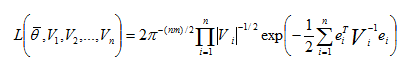
where:
n = number of experiments (i.e. observations)
m = number of measured response variables
Vi = variance-covariance matrix for the ith experiment
| Vi | = represents the determinant of Vi
ei = m x 1 residual vector that contains the differences between the measured values of the response variables and the values predicted by our mathematical process model.
![]() q
= the vector of
parameters to be estimated in our mathematical process model.
q
= the vector of
parameters to be estimated in our mathematical process model.
This expression is derived by substituting the residual vector, ei for the error vector in the multivariate normal probability density function (pdf). The error vector in the multivariate normal pdf contains the differences between the measured values of the response variables (the variables that we are fitting) and the true values. See Bard (1974) for details.
GPS-X also assumes that the measurement errors are independent from observation to observation and from response variable to response variable. This means that the variance-covariance matrices found in Equation 14.6 are diagonal but not necessarily equal.
In GPS-X the log-likelihood function is used instead of the likelihood function for mathematical convenience. Maximizing the log-likelihood function is the same as maximizing the likelihood function. The log-likelihood function is derived by taking the natural logarithm of Equation 14.6, as shown below:
Equation 14.7
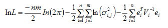
where:
![]() = variance of response j in experiment i
= variance of response j in experiment i
In this derivation, it is assumed that the variance of a response variable is not constant across all the observations. To take this into account, GPS-X uses the following expression for the estimated variance (Reilly et al., 1977):
Equation 14.8
![]()
where:
![]() = estimate of the variance,
= estimate of the variance,
![]()
wj = proportionality constant that will be called the standard deviation of the weighted residuals for response j
fi,j = value of response variable j predicted by the process model in experiment i
gj = heteroscedasticity parameter for response j
This expression relates the variability of response variable j to the magnitude of the predicted value for response j.
The heteroscedasticity parameter controls how the variance depends on the predicted values. This parameter is bounded between 0 and 2 and is continuous within this range. A value of 0 indicates constant absolute variability across all of the observations for response variable j. A value of 2 indicates constant relative variability across all of the observations for response variable j.
To determine the optimal value of wj, given the other adjustable parameters in the log-likelihood function, the estimated variance given by Equation 14.8 is substituted into Equation 14.7. The resulting equation is then differentiated with respect to wj and the derivative is set to zero, leading to the following expression:
Equation 14.9
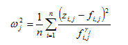
where:
![]() = measured value of response
j in experiment i
= measured value of response
j in experiment i
Substituting this expression into Equation 14.8 yields the estimate for the variance that accounts for non-homogeneous measurement errors:
Equation 14.10
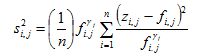
If Equation 14.10 is substituted into Equation 14.7, the log-likelihood function becomes:
Equation 14.11
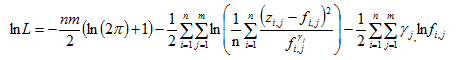
To allow for the possibility that the number of observations is different for each response variable, Equation 14.11 is re-written as (Steiner et al., 1990):
Equation 14.12
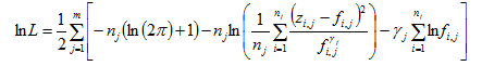
This is the function that is maximized by GPS-X to fit process models to measured data and obtain optimal parameter estimates. Equation 14.12 is a measure of the probability that the measurements were generated by the process model.
Note that the user can set the heteroscedasticity factors or have GPS-X estimate their optimal values for you.
As process models are generally nonlinear, the parameter values that maximize Equation 14.12 cannot be determined analytically. An iterative optimization method is required to maximize Equation 14.12. As mentioned earlier in this chapter, GPS-X uses the Nelder and Mead simplex method (Press et al., 1986) for optimization. This method is a type of direct search algorithm that does not require the calculation of partial derivatives. This is helpful when estimating parameters in systems of differential equations. The simplex method also has the advantage that it can handle objective functions containing discontinuities. This method is generally slower than derivative-based optimization methods, but can handle a greater variety of objective functions and is often found to be quite robust in finding solutions. The version of the simplex method implemented in GPS-X allows for bounds to be placed on the parameters.
Since the simplex method is designed for minimization, GPS-X minimizes the negative of Equation 14.12 to determine the optimal parameter estimates.
When there is only one target variable and the variance is constant across all observations (i.e. the heteroscedasticity parameter is zero), the sum of squares objective function is equivalent to the maximum likelihood objective function. For problems with more than one target variable, the sum of squares objective function is a special case of the maximum likelihood objective function that results if we make additional assumptions about the measurement errors. Our maximum likelihood objective function, given by Equation 14.12, is derived using the following assumptions:
· The measurement errors are normally distributed random variables with a mean of zero.
· For each target variable, the measurement errors are independent from observation to observation. Each target variable has its own variance which varies from observation to observation according to a power-law. The variances are unknown and are calculated as part of the optimization process.
· There is no correlation between different target variables
If we make the additional assumptions that all of the variances are
equal (i.e. all responses have same variance) and the variances do
not change from observation to observation (i.e. the
heteroscedasticities are all zero) then the maximum likelihood
function reduces to the sum of squares objective function in the
multi-response case. The assumptions used to derive the sum
of squares objective function in the multi-response case do not
apply in most practical situations. Therefore, it is
recommended that the maximum likelihood objective function be used
for calibration problems with more than one target
variable.
In this appendix, the solution report provided in the Log window after a GPS-X optimization run is discussed. The solution report provides the user with the solution found by the optimizer and a number of additional statistics that are valuable when doing parameter estimation. This report also may be printed to the stats.txt file. First we discuss the basic report and the detailed statistical report. This is followed by a summary on using the statistical tests and a discussion of over parameterization.
NOTE: In the solution report, the parameters are given generic names and are numbered according to the order that the parameters are listed in the Control window containing these parameters. For example, the parameter at the top of the Control window is labeled Parameter 1.
Many of the statistics in the solution report are organized according to target variable names. Generic target variable names are used and the names are numbered according to the order given for the target variables in the target variables form that is accessed by selecting Target Variables... from the Optimize drop-down menu. For example, statistics corresponding to the first target variable in the form are presented under the heading Target 1.
The basic solution report, which is printed to the Log window, includes the number of iterations required by the optimizer, the initial and final values of the objective function, the initial and final values of the parameters (i.e. the optimization variables), the heteroscedasticity parameter values, and a summary of the chosen optimizer settings. In addition, the statistics discussed below are provided if requested in the Optimizer form.
The gradient vector of the objective function is defined as:
Equation 14.13
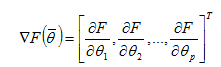
where:
F = the objective function
θ1, 2 / θp = the optimization variables
In the case of
parameter estimation these variables are the parameters being
estimated. The vector ![]() contains
the optimization variables.
contains
the optimization variables.
The partial derivatives are calculated numerically using the following forward-difference formula:
Equation 14.14
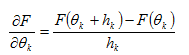
where:
k = 1
hk = the step or perturbation size
The step size is calculated using the following formula:
Equation 14.15
![]()
In Equation 14.15, the value of 10-7 is referred to as the finite-difference relative perturbation size in GPS-X and can be changed in the Derivative Information sub-section of the Optimizer form.
The gradient provided in the solution report is calculated at the solution. If the solution is a local minimum, the elements of the gradient vector should be close to zero. Because poor scaling of the parameters and the objective function can make the gradient appear large, the relative gradient is also reported. The elements of the relative gradient are calculated by scaling the gradient elements using the following equation:
Equation 14.16

The infinity norm of the relative gradient vector is also reported. If the solution is a local minimum, this norm should be close to zero.
The gradient is only reported when the report objective function gradient and Hessian switch in the Derivative Information sub-section in the Optimizer form is set to ON.
The model sensitivity coefficients express the local sensitivity of the process model to infinitesimal changes in the optimization variables (subset of the model parameters). They are the partial derivatives of the model with respect to the optimization variables. A sensitivity coefficient can be calculated for each target (i.e. response) variable with respect to each optimization variable at each data point. The sensitivity coefficients are calculated using the forward-difference approximation shown below:
Equation 14.17
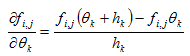
In this equation fi,j is the jth target variable at the ith data point. The step size is calculated in the same way as for the gradient.
The sensitivity coefficients are only reported when the report model sensitivity coefficientsswitch in the Derivative Informationsub-section in the Optimizer form is set to ON.
The Hessian is a matrix of second partial derivatives of the objective function with respect to the optimization variables. For the case of two optimization variables, the Hessian is defined as:
Equation 14.18
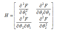
In GPS-X the elements of the Hessian are calculated using the Gauss-Newton approximation. For the sum of squares objective function, each Hessian element is defined as:
Equation 14.19
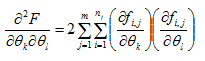
where:
m = number of target or response variables
nj = number of data points for target variable j
For the maximum likelihood objective function, Equation 14.5, each Hessian element is defined as:
Equation 14.20
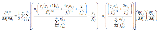
where γj is the heteroscedasticity of the jth response variable.
The variable ei,j is the residual and is defined as:
Equation 14.21
![]()
The variable zi,j is the measured value of response j at the ith data point.
The expressions in Equation 14.19 and Equation 14.20 were derived assuming that the response variables are equivalent to the state variables. Even if this is not the case, this is not a limitation because the sensitivity coefficients are being calculated using finite-differences. Therefore any dependencies in the responses are being taken into account.
The Hessian matrices for the other objective functions are not calculated because they cannot be approximated using the Gauss-Newton approximation. As a result, they require the calculation of second order sensitivities.
If any of the optimization variables are at their bounds, the elements of the Hessian involving these variables are zero.
The Hessian matrix is only reported when the report objective function gradient and Hessianswitch in the Derivative Informationsub-section in the Optimizer form is set to ON.
GPS-X calculates linear-approximation confidence limits for the parameter estimates using the variance-covariance matrix. For the sum of squares objective function, the variance-covariance matrix of the parameter estimates is defined as (Bard, 1974):
Equation 14.22
![]()
The matrix Ĥ-1 ![]() is
the inverse of the Gauss-Newton Hessian approximation to the sum of
squares objective function at the solution. The variable
s2 is the variance estimate for the measurement
errors and is defined as:
is
the inverse of the Gauss-Newton Hessian approximation to the sum of
squares objective function at the solution. The variable
s2 is the variance estimate for the measurement
errors and is defined as:
Equation 14.23

where
![]() is the value of the sum of squares objective
function at the solution, n is the number of data points
(total number considering all target variables), and p is
the number of parameters (i.e. optimization variables).
is the value of the sum of squares objective
function at the solution, n is the number of data points
(total number considering all target variables), and p is
the number of parameters (i.e. optimization variables).
For the maximum likelihood objective function, the variance-covariance matrix of the parameter estimates is defined as (Bard, 1974):
Equation 14.24
![]()
The matrix Ĥ-1 is the inverse of the Gauss-Newton Hessian approximation to the maximum likelihood objective function at the solution.
For both the sum of squares and the maximum likelihood objective functions, the 100(1-a) % confidence limits for parameter k are:
Equation 14.25
![]()
The variable t(n – p; a / 2) is the Student’s t-statistic, with n-p degrees of freedom, and a significance level of a / 2. In this case, n is the number of data points per response, except for the sum of squares objective function where it is the total number of data points. The variable a is the significance level for the parameter estimates. It is defined by the following expression:
Equation 14.26
![]()
where δ is the confidence coefficient. The confidence coefficient corresponds to the confidence level for confidence limits parameter found in the Confidence Limits sub-section of the Optimizer form. The default value is 0.95 so that by default GPS-X reports 95 percent confidence limits.
Equation 14.27
![]()
The confidence limits are only reported when the printing of confidence limitsswitch in the Confidence Limitssub-section in the Optimizer form is set to ON.
The detailed statistical report provides additional information that is helpful when doing parameter estimation. It allows the user to assess how well their model fits the measured data. The detailed statistical report is activated by setting the detailed statistical reportoption to ON in the Static sub-section of the Optimizer form. The statistics included in the detailed statistical report are discussed below.
The variance-covariance matrix is defined by Equation 14.22 for the sum of squares objective function and by Equation 14.24 for the maximum likelihood objective function. This matrix contains the variances of the individual parameter estimates (diagonal elements) and the covariances between the different parameter estimates (off-diagonal elements). Parameters with large variances may be unnecessary.
The elements of the correlation matrix are calculated as follows:
Equation 14.28
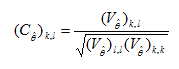
where
![]() is the (k, l) element of the
variance-covariance matrix.
is the (k, l) element of the
variance-covariance matrix.
By definition, the elements of the correlation matrix are always between zero and one. Unless some parameters are on their bounds the diagonal elements are always equal to one. The off-diagonal elements indicate the degree of correlation between pairs of parameters. A large off-diagonal element indicates a high degree of correlation between a pair of parameters. This provides evidence that some of the parameters in the model are unnecessary and the model is over parameterized. This may indicate that the model is not adequate for the task at hand or that the data do not provide enough information to allow estimation of all of the model parameters (Draper and Smith, 1981).
The variance-covariance and correlation matrices are only reported when the printing of confidence limitsswitch in the Confidence Limitssub-section in the Optimizer form is set to ON.
This is a statistic often reported by linear least squares packages. In GPS-X it has been modified to handle nonlinear maximum likelihood problems with heteroscedasticity. The statistic, adapted from Steiner et al. (1990), is calculated as follows for each target variable:
Equation 14.29
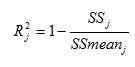
It is multiplied by 100 to get a percentage. The variable SSj is the weighted residual sum of squares for response j and is defined by:
Equation 14.30
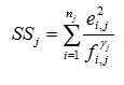
The variable SSmeanj is the total weighted sum of squares corrected for the mean and is defined below:
Equation 14.31
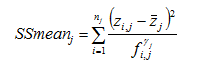
where ![]() is a weighted average of the measured values
for response j and is calculated as:
is a weighted average of the measured values
for response j and is calculated as:
Equation 14.32
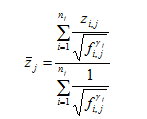
The overall variation explained is calculated as:
Equation 14.33
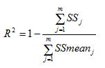
The % variation explained is not a model adequacy test but is useful because it shows how much of the variation in the data is accounted for by the fitted model. This test is only reported when the maximum likelihood or sum of squares objective functions are used.
This test involves testing the null hypothesis that all the model parameters are zero against the alternative hypothesis that all the parameters are not zero.
The following sum of squares ratio is calculated for each response variable:
Equation 14.34
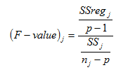
where SSregj is the weighted regression sum of squares for target variable j and is defined by:
Equation 14.35
![]()
The sum of squares ratio follows an F-distribution if the errors in the measurements are independent, normally distributed random variables and if the model parameters are all zero.
GPS-X reports the F-value for each target variable and reports the
probability that it is from an F-distribution with p-1 and
![]() degrees of freedom. If the probability is
larger than the chosen significance level it provides evidence that
the parameters are all zero and the regression is not significant
for the corresponding target variable. The significance level is
entered in the General Data > System > Parameters >
Optimizer form in the Significance of the Regression
sub-section.
degrees of freedom. If the probability is
larger than the chosen significance level it provides evidence that
the parameters are all zero and the regression is not significant
for the corresponding target variable. The significance level is
entered in the General Data > System > Parameters >
Optimizer form in the Significance of the Regression
sub-section.
If the probability value is smaller than the significance level it indicates that the F-value does not follow an F-distribution and therefore we accept the alternative hypothesis that the model parameters are not all zero. In this case the regression is significant for the corresponding target variable and the variation explained by the regression is greater than expected by chance. For a model to be useful for predictive purposes the F-values should be large and the probability values should be close to zero.
GPS-X provides messages that summarize the results of the significance test. The significance test is based on linear regression theory and is only approximate for nonlinear models.
This test is only reported when the maximum likelihood or the sum of squares objective functions are used.
This test determines whether the variance of the residuals is acceptable compared to the user supplied estimate of the measurement variance or the measurement variance calculated using replicate measurements. This serves as a model adequacy test.
For each target variable, the following sum of squares ratio is calculated:
Equation 14.36
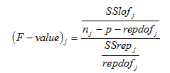
The variable SSrepj is the weighted replication sum of squares for target variable j and is calculated as:
Equation 14.37
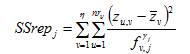
Where n is the number of independent variable values for
which there are replicates, nrv is the number of
replicates for the vth value of the independent variable,
![]() is the mean of the replicate
measurements corresponding to the vth variable,
zuy is the uth replicate measurement
corresponding to the vth variable, and fvj
is the predicted value of response variable j corresponding
to the vth value of the independent variable.
is the mean of the replicate
measurements corresponding to the vth variable,
zuy is the uth replicate measurement
corresponding to the vth variable, and fvj
is the predicted value of response variable j corresponding
to the vth value of the independent variable.
The variable repdofj is the degrees of freedom for the weighted replication sum of squares for target variable j. It is defined as:
Equation 14.38
![]()
As mentioned earlier, in this chapter, repeat measurements are inserted into GPS-X by placing measurements very close together in time in the .dat file. See the previous Lack of Fit Sub-Section, located in this chapter, for details.
The weighted lack of fit sum of squares for the jth target variable, SSlofj, is calculated as:
Equation 14.39
![]()
As mentioned in this chapter, the user also can provide the replication sum of squares and the replication degrees of freedom in the lack of fit sub-section of the Optimizer form. In order for these values to be used by GPS-X, the replication sum of squares option in the Lack of Fit sub-section of the Optimizer form must be set to User Supplied.
The sum of squares ratio or F-value follows an F-distribution if the errors in the measurements are independent, normally distributed random variables and if the weighted lack of fit sum of squares is not much larger than the weighted replication sum of squares.
GPS-X reports the F-value for each target variable and reports the probability that it is from an F-distribution with nj – p ‑ repdofj and repdofj degrees from freedom. If the probability for a certain target variable is smaller than the chosen significance level, it indicates that there is a lack of fit associated with this target variable. The significance level is entered in the General Data>System>Parameters>Optimizer form in the Lack of Fit sub-section.
GPS-X provides messages that summarize the results of the lack of fit test. The lack of fit test is based on linear regression theory and is only approximate for nonlinear models.
This test is only reported when the maximum likelihood or the sum of squares objective functions are used and the lack of fit switch in the Lack of Fit sub-section in the Optimizer form is set to ON.
The observed values are the measured target variable values provided in the .dat file. The predicted values are the target variable values calculated by the model that correspond to the observed values (i.e. they are calculated at the same points in time).
The % errors are useful for detecting any large discrepancies between the model and the measured data. The % error statistic is calculated as follows:
Equation 14.40
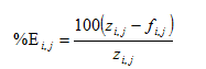
where %Ei, j is the percent error between zi, f and fi,j
As discussed earlier, the residuals are defined as:
Equation 14.21
![]()
They are an estimate of the error in the measurement, assuming that the model is correct.
The weighted residuals and standardized residuals are only reported when the maximum likelihood objective function is used. The weighted residuals are defined as:
Equation 14.41
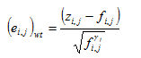
These are scaled residuals that are not as dependent on the magnitude of the measurements and the predicted values as are the unscaled residuals.
The standardized residuals are defined as:
Equation 14.42
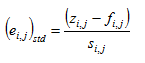
The variable Si,j is the estimated variance of response j for the ith data point and is defined in Equation 14.10.
The standardized residuals and their associated plots can be used to check whether the residuals are independent and normally distributed. This assumption is fundamental to the development of the maximum likelihood objective function used in GPS-X. The standardized residuals are normalized and should have a mean of zero and a variance of one if the residuals are normally distributed.
To check for violation of the independence assumption, the standardized residual plots should be examined for any noticeable trends. The presence of trends provides evidence of serial correlation. Serial correlation occurs when residuals taken in sequence are correlated with each other.
To check the assumption that the errors are normally distributed, the standardized residual plots should be examined to see if the residuals are randomly scattered about zero. In addition, the values of the standardized residuals should be examined to check whether approximately 95 percent of the residuals lie between +2 and -2.
The standardized residual plots are scaled to fit in the Log window. The largest standardized residual for each response variable is represented by the maximum number of " * " characters, which is seven. The remaining standardized residuals for a response variable are scaled relative to this maximum residual for the purposes of calculating how many " * " characters to print. You should consult the actual values of the standardized residuals provided in the Log window to determine whether the actual magnitudes of the residuals for a response variable are large.
If the assumption that the residuals are independent and normally distributed is violated it provides evidence that our model is inadequate to represent the experimental data. If the process model structure is correct, it should account for the non-random variability in the data.
The assumption that the residuals should be independent if the measurement errors are independent is not strictly correct but is fine for practical purposes. The residuals are always correlated to some extent as a result of the fact that there are n measurements but only (n - p) degrees of freedom, where p is the number of parameters to be estimated (Draper and Smith, 1981).
The Portmanteau test is used to detect trends in the weighted residuals. If trends are present, the residuals are not independent. This violates one of the assumptions of the maximum likelihood method and indicates that the model does not account for all of the non-random variability in the data. The Portmanteau test is designed for data taken in sequence (e.g. time or space).
The Portmanteau statistic for response variable j is calculated as the number of observations times the sum of the squared autocorrelations between the weighted residuals up to a certain number of time lags (Brockwell and Davis, 1996):
Equation 14.43
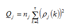
where nj is the number of data points for response j, τ is the number of time lags, and ρj(k) is the sample autocorrelation among the weighted residuals up to lag k for response j.
The sample autocorrelation is defined as:
Equation 14.44
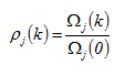
where Ωj(k) is the sample auto covariance function between the weighted residuals up to lag k for response j and is defined as:
Equation 14.45
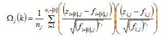
The sample autocorrelations are approximately independent, normally distributed random variables with mean zero and a variance of 1/nj if the weighted residuals are independent and identically distributed (Brockwell and Davis, 1996). This approximation gets better as the number of measurements increases. Although the residuals themselves are not necessarily identically distributed (they can have different variances), the weighted residuals should be identically distributed because they are scaled.
If the sample autocorrelations for a response variable are
independent and normally distributed as mentioned above, then the
variables ![]() should
should![]() be
independent and normally distributed with mean zero and variance
one. Since the Portmanteau statistic is a sum of squares of these
variables, it is distributed as a chi-squared variable.
be
independent and normally distributed with mean zero and variance
one. Since the Portmanteau statistic is a sum of squares of these
variables, it is distributed as a chi-squared variable.
GPS-X reports the Portmanteau statistic for each target variable and reports the probability that it is from a chi-squared distribution with degrees of freedom. If the probability for a certain target variable is smaller than the chosen significance level it provides evidence of a trend in this target variable's weighted residuals. The significance level is entered in the General Data > System > Parameters > Optimizer form in the Portmanteausub-section.
GPS-X provides messages that summarize the results of the Portmanteau test. This test is only reported when the maximum likelihood or the sum of squares objective functions are used and the portmanteau test on weighted residualsswitch in the Portmanteausub-section in the Optimizer form is set to ON.
See Table 4‑1 for a summary of how to use the statistics given in the solution report to assess the adequacy of the fitted model. Keep in mind that many of the tests become more reliable as the number of measurements increases. Even if the tests indicate that the model is not adequate, it does not mean that you cannot use the model. A visual inspection of the plots provided by GPS-X, showing the measured values and the predicted values, may indicate that the model captures the major trends in the data. This is often good enough for practical purposes as it may only be important to model certain aspects of a physical system.
Overparameterization occurs when there are more parameters in the process model than necessary to fit the data. This situation leads to correlations between model parameters as mentioned earlier in the context of the correlation matrix. As a result, the objective function near the solution to the parameter estimation problem has elongated contours and the solution is not very sensitive to changes in certain parameters.
The user should be careful when choosing the adjustable parameters in a parameter estimation run. The model should be sensitive to these parameters. It is often not practical to select the entire model parameters as optimization variables because this slows the optimization process, and will likely result in meaningless values for certain model parameters. It is preferable to choose only those parameters that have the greatest affect on the mismatch between the model and the data. See the Sensitivity Analysis chapter in the GPS-X User's Guide for details on how to conduct a sensitivity analysis of your model using GPS-X before doing a parameter estimation run.
Table 14‑1 - Summary of How to Use the Statistical Tests
|
Statistic |
How to Interpret |
|
Confidence Limits |
If the confidence limits on a parameter include zero it indicates that this parameter is not significant to the model. |
|
Correlation Matrix |
Large off-diagonal elements (close to one) suggest that certain parameters are correlated. |
|
Significance of Regression Test |
Probability values larger than the significance level indicate that the variation explained by the regression is less than expected by chance. |
|
Lack of Fit Test |
Probability values smaller than the significance level provide evidence for a lack of fit in the fitted model. |
|
Standardized Residuals |
The majority of standardized residuals should be between +2 and -2. |
|
Standardized Residual Plots |
The residuals should be randomly scattered about zero without any noticeable trends. |
|
Portmanteau Probability |
Probability values smaller than significance level suggest that the residuals are correlated. |
Bard, Y. A., Nonlinear Parameter Estimation. Academic Press, New York (1974).
Brockwell, P. J. and Davis, R. A. Introduction to Time Series and Forecasting. Springer-Verlag, New York (1996).
Draper, N. R., and Smith, H. Applied Regression Analysis. John Wiley & Sons, (1981).
Edgar, T. F. and Himmelblau, D. M. Optimization of Chemical Processes. McGraw-Hill, (1988).
Press, W. H., Flannery, B. P., Teukolsky, S. A., and Vetterling, W. T. Numerical Recipes: The Art of Scientific Computing. Cambridge University Press, New York (1986).
Reilly, P. M., Barjramovic, R., Blau, G. E., Branson, D. R., and Saverhoff, M. J. Guidelines for the Optimal Design of Experiments to Estimate Parameters in First Order Kinetic Models. Can. J. Chem. Eng., 55, 614 (1977).
Steiner, E. C., Rey, T. D., and McCroskey, P. S. SimuSolv Reference Guide. The Dow Chemical Company, Midland, MI, Vol. 2 (1990).
Dochain D. and Vanrolleghem P.(2001) Dynamic Modelling and estimation in wastewater treatment Processes, IWA Publishing, London, UK
Hauduc H, Neumann M. B., Muschalla D., Gamerith V., Gillot S. and Vanrolleghem P. (2011), Towards quantitative quality criteria to evaluate simulation results in wastewater treatment- A critical review, 8th IWA symposium on systems analysis and integrated assessment, Watermatex, pp 37-49
From MBR supplementary:
Membrane-Coupled Activated Sludge System: The Effect of Floc Structure on Membrane Fouling. Separation Science and Technology, 34(9), pp.1743-1758.
Choi, S., Yoon, J., Haam, S., Jung, J., Kim, J., Kim, W. (2000). Modelling of the Permeate Flux during Microfiltration of BSA-Adsorbed Microspheres in a Stirred Cell. Journal of Colloid and Interface Science, 228, pp. 270-278.
Garcia, G.E., Kanj, J. (2002). Two Years of Membrane Bioreactor Plant Operation Experience at the Vejas Tribe Reservation. Proceedings of the Water Environment Federation’s 75th Annual Technical Exhibition and Conference, September 28th – October 2, Chicago, Illinois.
Günder, B. (2001).The Membrane-Coupled Activated Sludge Process in Municipal Wastewater Treatment. Technomic Publishing Company, Lancaster, PA, USA.
Merlo, R.P., Adham, S., Gagliardo, P., Trussell, R.S., Trussell, R. (2000). Application of Membrane Bioreactor Technology for Water Reclamation. Proceedings of the Water Environment Federation’s 73rd Annual Technical Exhibition and Conference, October 14 - 18, Anaheim, CA.
Shin, H-S., Lee, W-T., Kang, S-T. (2002). Formation of Dynamic Membrane in Submerged Membrane Bioreactors (MBRs). Proceedings of the Water Environment Federation’s 75th Annual Technical Exhibition and Conference, September 28th – October 2, Chicago, Illinois.
Wallis-Lage, C., Steichen, M., deBarbadillo, C., Hemken, B. (2005). Shopping for an MBR – What’s for sale? Water Environment & Technology, 17(1), pp. 31-35.
The simulation results from dynamic wastewater treatment plant models are usually compared to the measured time-series datasets during model calibration and validation studies. Typically, the comparison between the dynamic simulation results and the time series measured data is based on qualitative assessment that involves visual inspection. Although, visual inspection based qualitative assessment is useful method to check the fit between the measured data and simulation results, the methods does not help in differentiating between goodness of one simulation results over the others when many simulation results can pass the qualitative assessment. In such situations it may be more meaningful to use quantitative statistical criteria to select the results of one calibration parameter set over the other.
Considering the usefulness of quantitative statistical criteria in evaluating and improving the model calibration and validation, a set of selected statistical indices were implemented in the GPS-X v6.4. The direct calculation of statistical indices inside GPS-X will significantly reduce the efforts of exporting and manipulating the simulation and measured data for estimation of the statistical indices. The statistical measures implemented will be explained in following sections using the predicted and measured BOD data as shown in a typical GPS-X output graph (see Figure 15‑1).
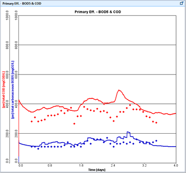
Figure 15‑1 – Typical Time Series Plot of Predicted and Measured Data
The time-series measured data is considered to contain, a time stamp at which the sample was collected and a value of the data. The time-series data could be available in a regular or irregular time intervals. The data measured at a wastewater plant could be from different type of sampling. The following data types are common:
1. Grab Data: The sample is collected at a specific time. The on-line data and data from grab samples belong to this category. The data point is fully defined by the time stamp and the measured value.
2. Time proportional composite data: Equal volumes of samples are collected at regular time intervals. These samples are mixed to give a composite sample. The data point is completely defined by the duration of composite and time interval for sample collection.
3. Flow proportional composite data: Equal volumes of samples are collected at equal volumes of wastewater treated. This means more number of samples is collected during high flow conditions and lower number of samples during the low flow conditions. These samples are mixed to give a composite sample. The data point is completely defined by the duration of composite and volume interval for sample collection.
As compared to the three measured data types indicated above, the raw simulation data produced by the wastewater models refers to a specific time and hence is similar to the Grab data type. Therefore, when simulation data is required to be compared with the composite measured data types (Type 2 and 3 above), a further processing of simulation data is necessary for meaningful comparison.
Considering the above discussion, depending on the type of the sample used for comparison, an equivalent sample data estimated using the simulation data in the statistical analysis. The type of sample can be specified in “Measured Data Type” section of the statistical setup menu (Figure 15‑2).
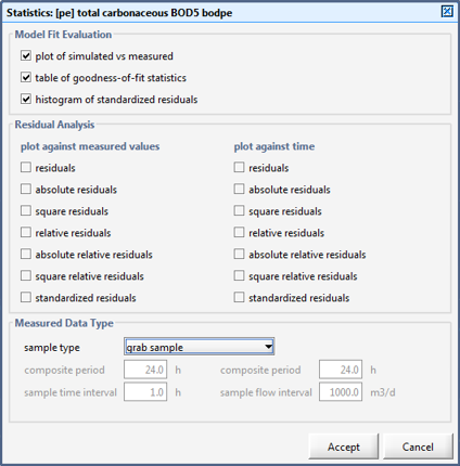
Figure 15‑2 - Statistical Analysis Set up Menu for Data Type, Output Plots and Table
The main objective in this first implementation is to focus on the most important statistical indices that may be helpful in quantitative assessment of model calibration and validation. A brief description of the statistical indices that are calculated for a given dataset is provided in Table 15‑1.
Table 15‑1 – Statistical Measures and Equations
|
No. |
Statistical Measure |
Equation |
|
1 |
Mean of Residuals |
|
|
2 |
Mean of Absolute Residual |
|
|
3 |
Mean of Squared Residual |
|
|
4 |
Absolute Maximum Residual |
|
|
5 |
Root of Mean Squared Residuals |
|
|
6 |
Mean of Relative Residual |
|
|
7 |
Mean of Absolute Relative Residual |
|
|
8 |
Mean of Squared Relative Residual |
|
|
9 |
Relative Volume Residuals |
|
|
10 |
Absolute Relative Volume Residuals |
|
|
11 |
Theil's Inequality Coefficient |
|
|
12 |
Nash-Sutcliffe (R2) |
|
|
13 |
Standard deviation of Residuals (SDR) |
|
|
14 |
Mean of Standardized Residuals |
|
Legend:
Oi = the observed (measured) value
Pi = the predicted (simulated) value
Om = mean of the observed (measured value)
n = number of data points
i = the ith observation
Ri = (Oi - Pi) = residual (error)
MR = Mean of Residuals
A typical GPS-X output showing the calculated statistical indices given quality indicator is as shown in Figure 15‑3.
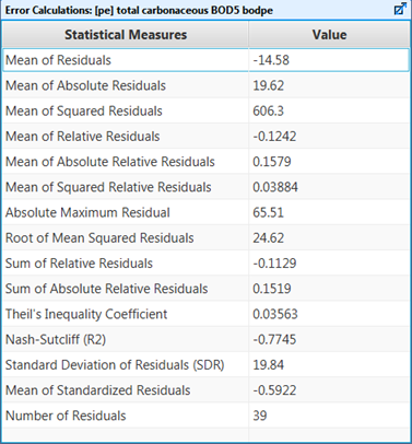
Figure 15‑3 - Summary of the Statistical Measures Calculated for a Time Series Dataset
In this plot the predicted values are plotted against the measured values. A 45 degree line is also placed on this graph to see the deviation of data points from this line. Assuming a perfect fit, the plotted data points will plot on the 45 degree line. Visual inspection of this plot can highlight the model biases and other systematic errors in the model. A typical output from GPS-X analysis is as shown in Figure 15‑4.
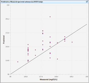
Figure 15‑4 - Predicted vs. Measured Data Plot
For a selected measured time series data, a number of residuals as show in Table 15‑2 are estimated. The calculated residuals are used for plotting against time or observed data. A histogram of the standardized residuals is also made available for evaluating the model fit.
Table 15‑2 – Types of Residuals
|
No. |
Criteria |
Equation |
|
1 |
Residuals |
|
|
2 |
Absolute Residual |
|
|
3 |
Squared Residual |
|
|
4 |
Relative Residual |
|
|
5 |
Absolute Relative Residual |
|
|
6 |
Squared Relative Residual |
|
|
7 |
Standardized Residuals |
|
A histogram of the standardized residuals are plotted to check the assumption that the errors are normally distributed. The histogram of standardized residual may also help to inspect if the residuals are randomly scattered about zero and to approximately 95 percent of the residuals lie between +2 and -2. A histogram produced for the BOD dataset is as shown in Figure 15‑5.
The estimated residuals can be plotted against the measured data point to see trends and biases in model outputs. A typical output of this type of plot is as shown in Figure 15‑6.
For identifying trends in estimated residuals, the time plots of the residuals may be useful. The model predictability may be affected some specific time based events and these plots may be of help to identify time periods of special events (rain fall, plant maintenance etc.) where the plant operation conditions are not captured adequately in the model. A typical output for this type of plot is as shown in Figure 15‑7.
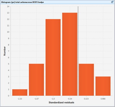
Figure 15‑5 - Histogram of Standardized Residuals
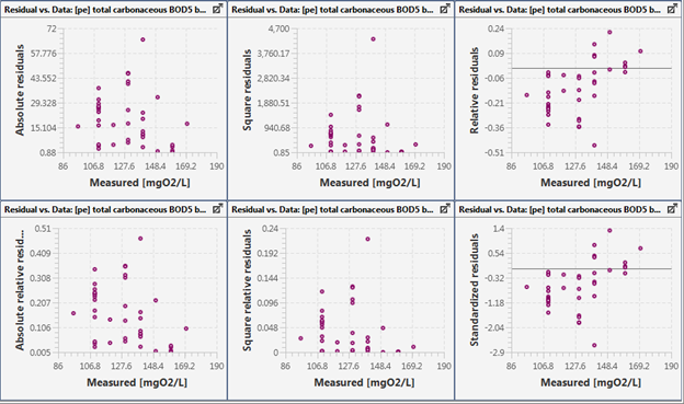
Figure 15‑6 - Residuals Plotted against the Observed Data
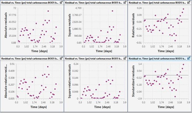
Figure 15‑7 - Residuals Plotted against Simulation Time
This feature allows the user to set the speed of the simulation to real time or to a multiple of real time. This is useful in on-line SCADA applications or for operator training in which GPS‑X acts as a virtual plant.
The parameters for this feature
can be accessed at the bottom of the
General Data > System > Parameters > Simulation
Tools Settings form (Figure 15‑8), and select
the More… button in the On-line Operation
sub-section. The Real Time Synchronized Mode sub-section
contains the parameter that will switch the real time clock
ON or OFF. When the real time clock is ON, the
simulation speed is equal to a multiple of real time. The
multiplication factor used is specified by the Real Time
Accelerator Factor. (i.e. setting the accelerator factor to 24
causes one simulation day to take one real hour). Note, the real
time clock feature forces the Communication interval to be
equal to one second.
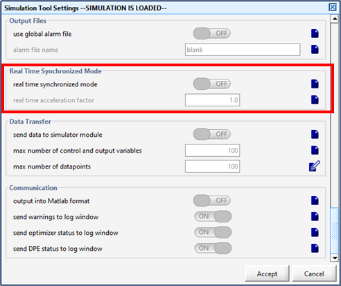
Figure 15‑8 - Real Time Clock Parameters
The steady-state solver used in GPS-X is a robust routine based on a direct search algorithm (that is, no gradients are used). Sometimes, the steady-state convergence appears slow or diverges due to a problem in the way that the model is set up. For example, if the underflow rate from a settler is too low, that settler will begin to fill up with solids. Since the concentration ranges of solids in the ten layers become large, the changes in these layers between loops of the steady-state solver also become large which may cause slow convergence or divergence.
In all cases of poor convergence, the user should closely examine all the unit processes for proper specification. The easiest way to do this is to examine the dsum# variable associated with each unit process where # represents the overflow stream label. You can do this by issuing the display command in the Command line of the Simulation Control window. The sum of the individual dsum values equals the dsum value displayed in the Log window. Having done that, there are a number of parameters associated with the steady-state solver that can be fine-tuned.
The forms shown in Figure 15‑9 and Figure
15‑10 are accessed by selecting
General Data > System > Parameters > Steady-State
Solver Settings. The parameters in these forms are
described below.
The first menu item, number of retries on iteration indicates the number of times the steady-state solver will try to reach convergence if it fails.
The error limit on individual variables is a tolerance below which the steady-state ignores a variable. If the steady-state solver is making changes to a state variable that become smaller than this tolerance, the solver will ignore the variable, assuming it is at steady-state.
When the solver achieves a sum of state variable derivatives below the iteration termination criteria, a steady-state convergence is triggered. The default value is 10.0, but in some systems it may need to be increased when in single precision.
The contract constant and expand constant refer to the step size made by the steady-state solver between iterations. A larger step is taken if an improvement is found, while a smaller step is taken if no improvement is found. The performance of the steady-state solver can be greatly affected by these parameters. The expansion factor is limited to the maximum step size in one iteration. This maximum step size is dampened as the steady-state solution is reached. The damping factor on final approach will control the damping effect. A zero value means no damping; while a value of 1.0 means that the maximum step size is limited to one tenth of the maximum step size.
The initial step size that the steady-state solver takes is governed by the initial perturbation parameter. This number is normally set smaller than the maximum step size to prevent a poor initial guess by the solver.
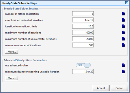
Figure 15‑9 - Steady State Parameters
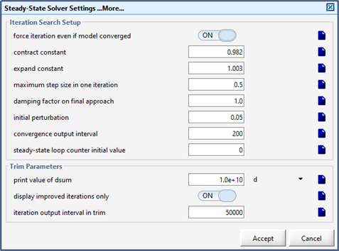
Figure 15‑10 - More Steady-State Parameters
The next four items shown in these forms deal with other termination criteria and output control. The status of the solver is printed at a frequency controlled by the convergence output interval, while the steady-state loop counter initial value specifies which iteration loop will be first printed to the simulation Log window. The maximum number of iterations limits the steady-state solver to attempting only this many iterations. The loop counter is reset after each retry. Another steady-state termination criterion is the maximum number of unsuccessful iterations which will cause the steady-state solver to terminate if an improvement in the value of the sum of the derivatives is not made within this number of loops.
The trim parameters shown here refer to the output of the ACSL trim function. This is an alternative steady-state solver, which uses the Jacobian matrix for accelerated searches. However, this gradient type routine was not found to be very robust with the large models encountered within GPS-X.
The Advanced Steady-State Parameters sub-section contains parameters that are used to enhance and refine the contraction process for each state variable. The maximum concentration bound for each state variable are found in the More… button menu.
The numerical issues discussed in this chapter are important because the success of a simulation depends on the input data and the models and on the numerical solver used to do the calculations.
Any modeller using dynamic simulation should have an understanding of the underlying numerical methods used to solve the equations to properly interpret the results. Understanding the numerical methods used will help to identify problems that are numerical in nature.
The choice of which numerical solver to use is important. There are
several numerical integration methods available in GPS-X. The
numerical solver can be set in the Simulation Control window
or can be saved into a scenario or the layout by setting it in
General Data > System > Input Parameters > Dynamic
Solver Settings and scrolling down to the Integration
Settings sub-section (Figure 15‑11).
Generally, the default integration method, Runge-Kutta-Fehlberg (2), works very well for most models; however, there are situations where the solver may need to be changed. In general the trade-off is between numerical accuracy and simulation speed. The fixed step algorithms (i.e. Euler, Runge-Kutta (1), and Runge-Kutta (2)) are faster than the variable step algorithms (i.e. Adams-Moulton, Runge-Kutta-Fehlberg (1), Runge-Kutta-Fehlberg (2), Gear's Stiff, and Differential Algebraic Solver) but are not as accurate.
If the system is stiff then you may need to use the Gear's Stiff algorithm. A stiff system is one in which there are processes occurring at very different time scales (e.g., a very fast process such as the transfer of oxygen into a tank and a very slow reaction occurring at the same time).
In addition to the
numerical solvers, the user can change some of the numerical
parameters that control the simulations. Changing the default
parameters however requires extreme caution because in some cases
it may introduce errors in the results. The numerical parameters
are accessed by making the following selections:
General Data > System > Parameters >
Numerical. The form is shown in Figure
15‑12.
These parameters include bounds on flow, state variables, state derivatives, parameters, exponentials, and volumes. The parameters for the implicit solver (IMPL - used for solving implicit functions evaluated as residuals, where the residuals are reduced to zero) used in the exact code option can be set here. Some of the parameters are discussed in more detail in the sub-sections below.
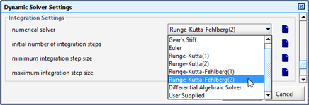
Figure 15‑11 – Integration Methods
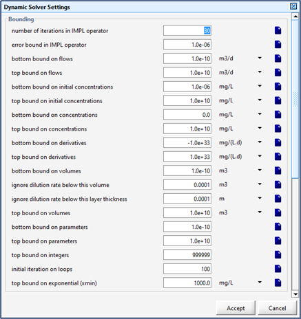
Figure 15‑12 - Numerical Parameters Form
If the liquid volume in a tank falls below the ignore dilution rate below this volume parameter value, then the dilution rate (defined as the inverse of the hydraulic residence time) will not be used to calculate the concentrations in the tank as would normally be done. In doing so, the speed of simulation is greatly increased. The same principle is applied to the settlers and SBRs where the dilution rate in a particular layer is ignored if the height of the layer is smaller than the ignore dilution rate below this layer thickness parameter value.
The parameter protect against division by zero is fixed and cannot be changed by the user. This parameter is used in all calculations involving division. It is used to ensure that the denominator in an expression is never equal to zero. For example, the DO switching function, used in many rate equations (shown below), includes the protection against division by zero parameter.
Equation 15.1
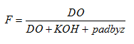
The parameters in the Speed sub-section of the Numerical form concern the pump flow rates used in all the objects. Since the switching of pumps on and off introduces sharp changes in the flows, the numerical integration routine may require a very small step size to reduce the numerical error. In some cases, these small step sizes will result in a very slow simulation. If the smooth pump discharge at discontinuitieslogical is turned ON (default is OFF), then the pumped flow rate is ramped up to the specified amount as follows:
Equation 15.2
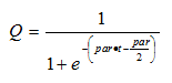
where:
Q = pumped flow rate (m 3/d),
par = smoothing factor,
t = smoothing period (d).
The smoothing function will only be applied to a user-specified percentage change (smooth at flow changes larger than). This allows the user the flexibility of smoothing only larger changes in a pump flow rate. The smoothing function will be applied to all pump flows in a layout including underflows, control splitters, etc. See Figure 15‑13 for an illustration of how the smoothing function affects the pumped flow.
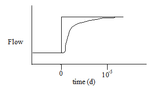
Figure 15‑13 - Smoothing Function
Although GPS-X allows the user to build very large and complex layouts, there are some restrictions. First, the simulation language used, ACSL, currently has a limit on the number of discrete blocks of code that can be specified. What this means to the user is that the number of automatic controllers for a given layout cannot exceed 25. Since a number of objects have built-in controllers (e.g., settler has a controller for both the pumped flow and underflow), the user can quickly use all the allowable discrete code blocks. To circumvent this problem, the user can select either the Big option, which combines all the automatic controller code into one discrete block, or the Big+ option, which disables all controllers. In selecting the Big option, the user can no longer specify the sampling time for each individual controller loop. One sampling interval will override the rest. This sampling interval (controller sampling time) is found under General Data > System > Parameters > Miscellaneous.
A trade-off exists between the speed of the simulation and the robustness and accuracy of the model under different conditions (e.g. sudden flow discontinuities or tanks emptying completely). GPS-X is configured such that the average user with a typical continuous flow activated sludge plant need not worry about the accuracy and the speed of the simulation. However, when dealing with more complex processes it may be necessary for the user to switch to a different integration algorithm or change the values of some numerical parameters to improve the accuracy or speed of the simulation. In general, robustness and accuracy are more important than simulation speed.
If you suspect that the simulation results are not accurate, you should first check that the physical dimensions of the process objects and the values of the process flows are reasonable. A numerical value may have been entered incorrectly.
If you are confident that the model parameters are reasonable then the next step is to determine whether a modelling simplification or numerical problem is leading to inaccurate results. Some helpful information is listed below:
· If you suspect that the simulation results are not accurate, you may wish to try the Exact code option. (Build > Code menu item). The Quick option (default) results in a faster simulation but is not as accurate when recycle flows are present. When the Quick option is used the recycle flows at each time step are simply the values taken from the previous time step. When the Exact option is used the recycle flows are calculated exactly using an implicit nonlinear equation solver. In most situations using the Quick option is acceptable, because the integration time steps are small and recycle flows usually don't change dramatically. In an application with a number of recycle flows and sudden extreme dynamic changes this simplification may cause some problems.
· The choice of integration algorithm (IALG) can have a significant effect on the output of the model. For a detailed description of the available integration algorithms consult the ACSL Reference Manual (contact Hydromantis for details). Generally, only variable step algorithms (i.e. Adams-Moulton, Runge-Kutta-Fehlberg(1), Runge-Kutta-Fehlberg(2), Gear's Stiff, and Differential Algebraic Solver) are acceptable for the simulation of highly dynamic systems. Try the Gear's Stiff algorithm if you suspect that your system is stiff (unless you are simulating an SBR or trickling filter, in which case only the Runge-Kutta-Fehlberg algorithms are allowed).
The Gear's Stiff routine is a self-tuning algorithm that adapts itself to rapidly changing derivatives - in some cases though it might require excessive simulation time to cross a discontinuity in the model. The Runge-Kutta-Fehlberg(1) algorithm is exactly the opposite - it is very forgiving for discontinuities, but experiences difficulties with steeper problems. A good compromise between these two solvers is the Adams-Moulton algorithm. It is very robust and does not give up easily but it is slower. The Runge-Kutta-Fehlberg(2) algorithm is almost identical to Runge-Kutta-Fehlberg(1), but is more robust.
·
It is possible to monitor the step sizes used by the integration
algorithm during a run. You can either print the values to the
Log window by entering the following command at the command
line in the Simulation Control window: output
truecssitg or place the variable truecssitgon an output
graph. You can select truecssitgfor display in the
General Data > System > Output Variables > General
program variables form (it is labeled as Average integration
step size). The average integration step size
(truecssitg) is calculated over each communication
interval. Start your simulation using a small
communication interval (~0.01 or less). Sharp drops in
truecssitg usually signal a discontinuity. Using the above
method, the Sum of absolute values of the
derivatives (dsum) can also be checked for
sharp changes.
· If your simulation is slow you can find which variable makes the simulation slow by selecting the Fullinfo option in the Options>Set up>Information menu of the Simulation Controlwindow, and running the simulation using either the dams-Moulton or Gear’s Stiff integration algorithms. The error summary displayed at the end of the run in the Log window will point to the variable that controls the step size.
· The integration of systems with low DO (dissolved oxygen) concentrations (in the range of a few dozen micrograms) is time consuming because the integration algorithm has to cut back on the step size or risk running into negative DO values.
· Sometimes the integration algorithms have difficulty at the start of a simulation. In such cases the initial concentrations of the state variables may be inappropriate, resulting in large initial derivative values. In this case the variable step integration algorithms keep cutting back on the step size to go over this initial bump. It may be helpful to use the steady-state solver to determine the initial conditions.
·
Simulation speed depends strongly on the values of the derivatives
of the state variables. You can reduce the absolute value of the
lower and upper bounds on the derivatives to speed up the
simulation of discontinuities by eliminating sharp peaks. These
bounds can be found in the
General Data > System >
Parameters > Dynamic Solver Settings form. The
best values to use depend on the system in question. Try plotting
the DO derivative (found in the Process Data menu for each object),
because this is the most sensitive state variable in most cases.
Get the maximum value during the run and then select the bounds to
be 50 percent of the highest value. Changing the bounds from the
default values (-1.e33 and 1.e33) can restrict the accuracy of the
integration.
· Sudden start-up or switching off of pumps (influent or other) can cause discontinuities in the derivatives, and as a consequence, a delay in the processing of the simulation. To prevent this, a smooth pump option is provided in the General Data > System > Parameters > Dynamic Solver Settings form, which starts and stops pumps smoothly. This is strictly intended as a numerical feature and does not try to simulate real pump discharges during transient periods. By default, the smoothing is not used. If you experience problems when pumps are turned off or on, try using smoothing.
· Check the Log window for any messages printed during the run.