Tutorial 3

Editing Layouts and Using Scenarios

Problem Statement

For this tutorial, consider a situation where the plant you developed in the second tutorial is expected to increased influent flows of differing qualities due to, for example, storm conditions. To control the quality, the plant needs an additional membrane filter and a disinfection unit.

Objectives

GPS-X makes it easy to build models to help you examine changes in plant design and operation.  This tutorial will show you how to use the layout editing tools such as Copy and Paste to make additions to the layout. Once the new model is built, the scenario features of GPS-X will be introduced.  Using scenarios, you can set up specialized data sets for comparing the performance of different units in the event of uneven flow distribution under both steady state and dynamic conditions.

When you are finished with this tutorial, you will have developed the ability to create and edit plant layouts and will have developed a better understanding of static data input and output in GPS-X.  You will be able to prepare simulation scenarios to test different hypothetical situations and be able to run the scenarios to test alternative plant designs or examine operational changes.

Expanding the Plant

1. Open the layout built in Tutorial 2 and save it as ‘tutorial-3’ using File > Save As...

2. Switch to Modelling Mode (if not already there) using the button on the top right-hand side of the screen.

3. Display the grid on the drawing board.  Select View > Display Grid from the main toolbar.

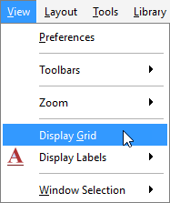
Figure 3‑1- Selecting Display Grid

4. Display a larger drawing area.  In order to expand on the layout, more space is required on the drawing board.  Open the Locator window under View > Zoom > Locator and outline a larger working area. Alternatively, the mouse wheel can be used to scroll out and the desired work area can be highlighted and then zoomed in on by using the Zoom to selection/plant button. This will allow you to place more objects on the drawing board. More details regarding use of the Locator are presented in Tutorial 1.

5. Move the Treated Water object by clicking and dragging out a box around the object. Then with the mouse button pressed on the object, drag the selected area to its new location on the drawing board (see Figure 3‑2).

6. Move the River Water Influent object by clicking and dragging the object to the left.

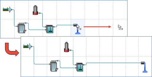
Figure 3‑2- Moving A Unit Process

7. Delete unneeded connections. You can delete a connection by right clicking on the connection and selecting Delete Connection.

Alternatively, you can delete the flow lines by placing the cursor at the initiation or terminal point of a flow line and dragging the flow line to an empty space on the drawing board. As soon as the mouse button is released you will be prompted to confirm the deletion of the flow line.

Delete the connection from the Neutralization Tank to the Treated Water object, and the connection between the River Water Influent object and the Membrane Filter. 

8. Add processes to the drawing board. From the Flow Combiner and Splitters group in the Process Table we will need one 2-Flow Combiner. From the Disinfection group in the Process Table we will need one Chemical Disinfection unit.

Position the objects so that the model resembles Figure 3‑3.

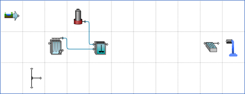
Figure 3‑3- Add a Combiner and a Disinfection Object

9. Copy the Membrane Filter. Using the Copy and Paste functionality in GPS-X, you can create an exact copy an object in the GPS-X layout including any input parameter changes you have made to the object.

First select the Membrane Filter in the GPS-X layout by clicking on it. When the cell containing the Membrane Filter is selected, it will be shaded light blue. Click the Copy button on the main toolbar to have a copy available in your GPS-X clipboard. Next, select where you would like to make a copy of the object by dragging out a small square in the drawing board cell. When a cell is selected, it will be highlighted light blue. Pressing the Paste button will paste a copy of the Membrane Filter and all its attributes in the new location.

Your layout should now look like Figure 3‑4.

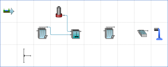
Figure 3‑4– Copy/Pasted Membrane Filter

	10. Flip the 2-Flow Combiner. To do this, select the combiner and press the Mirror button on the main toolbar.
	11. Rotate the 2-Flow Combiner. To do this, select the combiner and press the Rotate button on the main toolbar.

12. Connect all objects and label all units and streams.  The last step of the plant expansion is to connect all the objects and label them appropriately as seen in Figure 3‑5 and Table 3‑1.

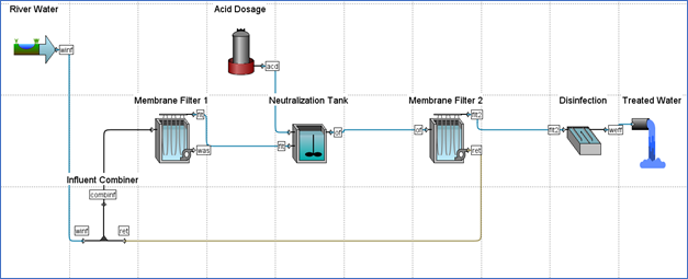
Figure 3‑5- Processes and Streams Labelled Properly

NOTE: The colors of the flow lines each convey a specific meaning about the properties of the stream. 

Brown lines are used to represent the flows of wastewater/sludge. An example of this is the sludge leaving a membrane filter

Black lines are used to represent any streams where you are unable to tell what the outputs will be when the object is selected. An example of this is the combiner object. 

Blue lines are used to represent any flows of water/treated water. An example of this is the river water influent.

Table 3‑1- Process and Stream Labels

Unit	Label
River Water Influent	Label: River Water Influent: winf
Membrane Filter 1	Label: Membrane Filter 1 Filtrate: flt Concentrate: was
Neutralization	Label: Neutralization Tank Overflow: of
Acid Dosage	Label: Acid Dosage Influent: acd
Membrane Filter 2	Label: Membrane Filter 2 Filtrate: flt2 Concentrate: ret
Chemical Disinfection	Label: Disinfection Output: weff
2-Flow Combiner	Label: Influent Combiner Output: combinf
Treated Water	Label: Treated Water

13. Add a note to a process.  Sometimes it is useful to make a note to remind yourself about certain details or reasons for changing something.  These notes are just for your own reference and do not affect the simulation in any way.

Here, we will add a note to the Membrane Filter 2 unit.  Right-click on it and chooseNote… from the popup menu.  A blank window will appear in which description of the unit can be typed. Click Accept to close the Note window.

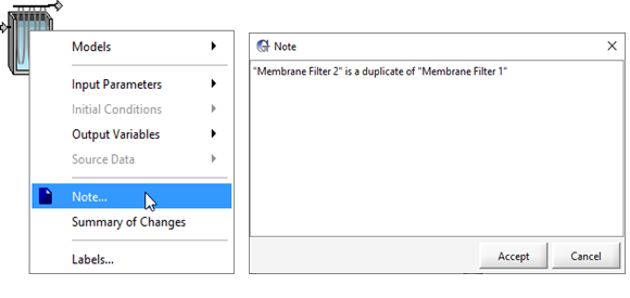
Figure 3‑6  - Add a Note to a Process

14. Save the layout. Press the Save button on the main toolbar.

Using Scenarios

When organizing simulation runs it is useful to start with a base set of data, and then create one or more separate cases, which are modifications to the base data set. These cases are referred to as scenarios in GPS-X.

You can create any number of scenarios and in each scenario, you can specify the changes to the model parameter(s) which define that scenario.  Those changes are saved so that they can be restored at any point in the future.

Creating and using scenarios is done in Simulation Mode.

In this section of the tutorial, we are going to use scenarios to investigate the effects of changing the following model parameters:

· Influent flow: to simulate the surges in the influent flow rate

· Disinfection settings: to manually control surges in the influent conditions

15. Switch to Simulation Mode using the button at the top-right of the screen.

16. Create a new scenario by selecting Newfrom the Scenario menu on the Simulation Toolbar (at the bottom of the main window).

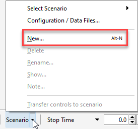
Figure 3‑7- Create a New Scenario

17. Type in a name for your new scenario (eg. “Surge Flow”) and Accept the form.

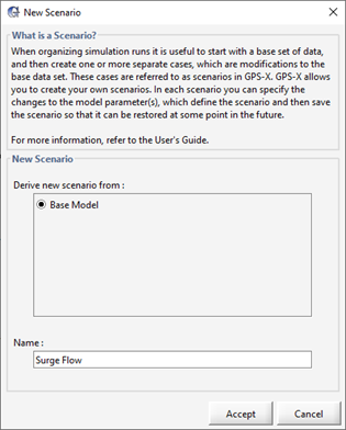
Figure 3‑8- Name the Scenario

You will notice that the name of the active scenario is displayed under the Start button on the Simulation Toolbar.

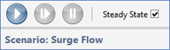
Figure 3‑9- Scenario Name Display

NOTE:  You can change the active scenario by selecting it from the Scenario > Select Scenario list.  The “Base Model” scenario is the base case where all the model parameters are set to the values defined when the model was built. If you return to modelling mode and make changes to the Base Model Parameters, these changes will be applied to all scenarios where that parameter has not been directly specified.

18. Add some parameter changes to the scenario.  In this case, we will change the influent flowrate and type.

While remaining in Simulation Mode, access Flow > Flow Data from influent objects process data menu (ie. right-click on the object).

Change the Flow Type to Sinusoidal and change the Influent Flow to 5000 m3/d.

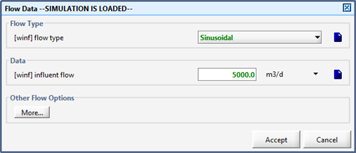
Figure 3‑10- Changing Parameters in a Scenario

You will notice that changes made in a scenario are highlighted in green to indicate they have only been changed in the current scenario.

Accept the form.

19. Verify the parameter changes made in the scenario. Any ways a scenario has been modified from the base scenario can be viewed by selecting Show… option in the Scenario menu on the Simulation Toolbar.

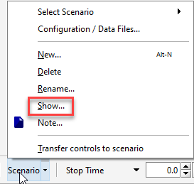
Figure 3‑11- Show Changes Made to the Active Scenario

This window will show a summary of any variables that have been changed in the current scenario. The value that the variable was assigned when the model was built is shown in the grayed-out box. If any of the variables changed in this scenario appear on an input controller, an icon will appear next to the variable name to indicate the input controller.

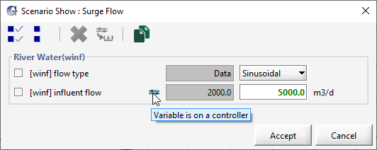
Figure 3‑12- Summary of the Changes made in the Active Scenario

Parameter changes in a given scenario can be directly edited in this menu by adjusting the setting of the box that is not grayed out. Additionally, any unwanted changes can be returned to their default value by checking the box next to the parameter name and pressing the Remove button in the toolbar.

Accept the form.

20. Create a new input control tab. Press the New Tab button on the controls toolbar to create a new input control tab. Double click on the tab name to change it (i.e. Flow Controls)

21. Create an input control (slider type) for the Influent Flow as described in the Creating Input Controls section of Tutorial 2. Set the minimum and maximum values to 0 and 12,000 m3/d respectively.

22. Create an Input Control (slider type) for the Chlorine dosage used in the Chemical Disinfection object. The Chlorine Dosage can be accessed by right clicking on the Chemical Disinfection object and selecting Input Parameters> Feed Chemical. Set the minimum and maximum values to 0 and 10 mg/L respectively.

Create an Input Control (slider type) for the total coliform dosage before disinfection in the Chemical Disinfection object. The total coliform dosage before disinfection variable can be accessed by right clicking on the Chemical Disinfection object and selecting Input Parameters > Operational. Set the minimum and maximum to 0 and 25,000,000 MPN/100mL respectively.

23. Create X-Y graphs for the log inactivation of microorganisms and for the total coliform count after disinfection. Create a separate graph for each of these variables. In each case, the output variable be found in Output Variables > Disinfection menu of Disinfection object. Display each variable on its own graph.

24. Autoscale the y-axis on each of the graphs and rename them appropriately.

25. Rename the new output tab to “Effluent Microorganisms”

26. With the steady state box checked, run a 1-day dynamic simulation.

27. Increase the Influent Flow Rate to 8,500 m3/d and change the stop time to 2 days.

28. Resume the simulation using the Resume button (i.e. don’t restart the simulation) and let the simulation proceed until it stops.

29. Increase the Total Coliform Count Before Disinfection to 20,000,000 MPN/100mL and change the stop time to 3 days.

30. Resume the Simulation.

31. Increase the Chlorine Dosage to 8.0 mg/L and change the stop time to 4 days.

32. Resume the Simulation.

A set of typical results are shown in Figure 3‑13. These graphs show a surge in influent conditions and an attempt to correct them using an increased chemical dosage.

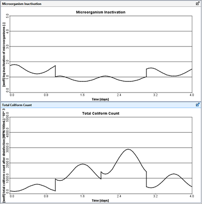
Figure 3‑13- Typical Results

Previous Next